import pandas as pd
url = "https://raw.githubusercontent.com/fahadsultan/csc272/main/data/elections.csv"
elections = pd.read_csv(url)Vectorized Operations
Vector based programming (also known as array based programming) is a programming paradigm that uses operations on arrays to execute tasks. This is in contrast to scalar based programming where operations are performed on individual elements of an array.
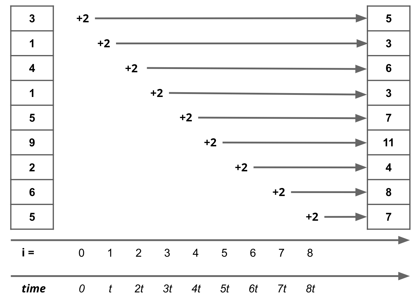
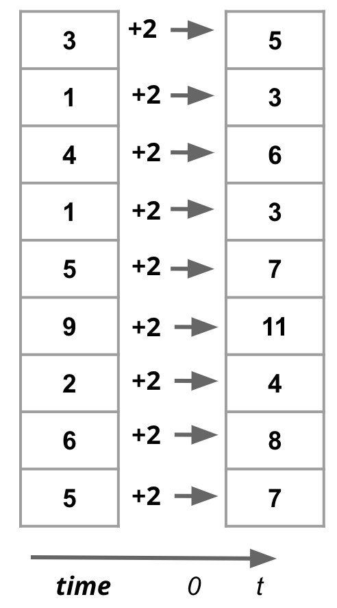
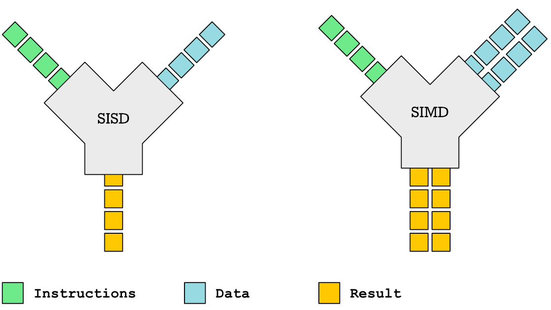
Vectorization operates at the level of individual instructions sent to a processor within each node. For instance, in the illustration shown here, the instruction is to add 5 to a column of numbers and copy the results to a new column B. With vectorization, all the data elements in that column are transformed simultaneously, i.e. the instruction to add 5 is applied to multiple pieces of data at the same time. This paradigm is sometimes referred to as Single Instruction Multiple Data (or SIMD).
We can think of vectorization as subdividing the work into smaller chunks that can be handled independently by different computational units at the same time.
In this course, we will be minimizing the use of loops.
 |
 |
| 1. Serial / Sequential Operations | 2. Vectorized Operations |
This is orders of magnitude faster than the conventional sequential model where each piece of data is handled one after the other in sequence.
Vectorized operations are also known as SIMD (Single Instruction Multiple Data) operations in the context of computer architecture. In contrast, scalar operations are known as SISD (Single Instruction Single Data) operations.
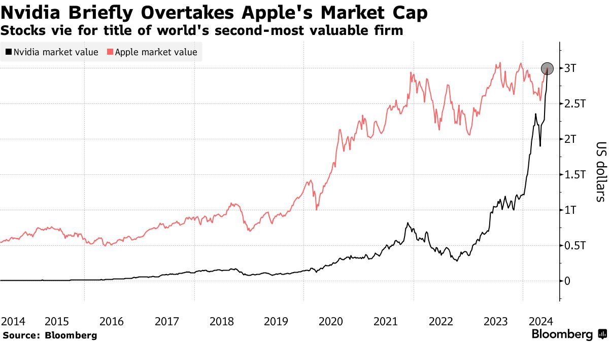
With vectorization, performing the same operation on a modern intel CPU is 16 times faster than the sequential mode. The performance gains on GPUs with thousands of computational cores is even greater. However, despite these remarkable performance benefits, most analytical code out there is written in the slower sequential mode. This is not a surprise, since until about a decade ago, CPU and GPU hardware could not really support vectorization for data analysis. So most implementations had to be sequential.
The last 10 years, however, have seen the rise of new technologies like CUDA from NVidia and advanced vector extensions from Intel that have dramatically shifted our ability to apply vectorization. Because of the power of vectorization, some traditional vendors now make claims about including vectorization in their offerings. But shifting to this new vectorized paradigm is not easy, since all of your code needs to be written from scratch to utilize these capabilities.
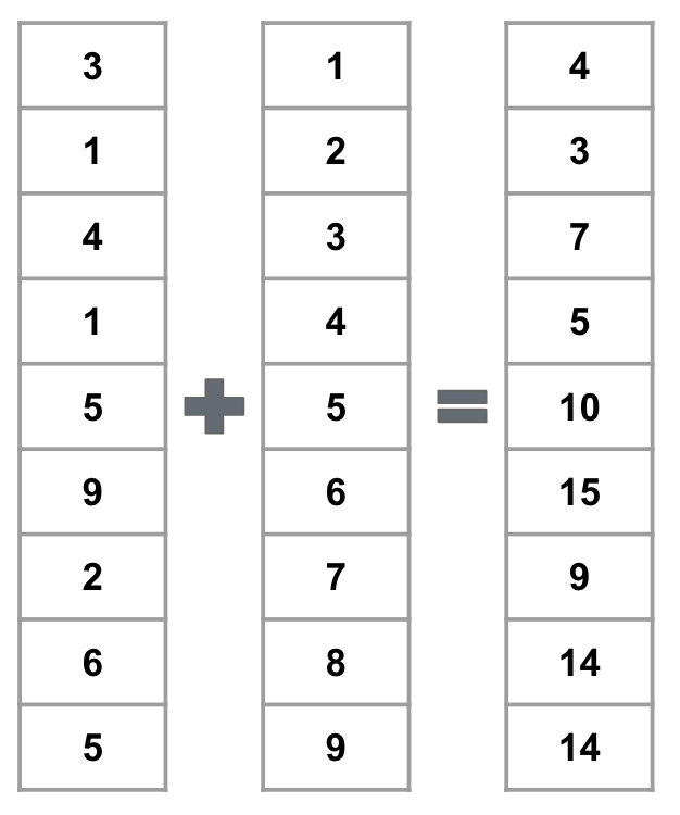
Vectorization can only be applied in situations when operations at individual elements are independent of each other. For example, if we want to add two arrays, we can do so by adding each element of the first array to the corresponding element of the second array. This is a vectorized operation.
However, for problems such as the Fibonacci sequence, where the value of an element depends on the values of the previous two elements, we cannot vectorize the operation. Similarly, finding minimum or maximum of an array cannot be vectorized.
Let’s read in the same elections data from the previous exercise and do some data manipulation and wrangling using pandas.
Data Alignment
pandas can make it much simpler to work with objects that have different indexes. For example, when you add objects, if any index pairs are not the same, the respective index in the result will be the union of the index pairs. Let’s look at an example:
s1 = pd.Series([7.3, -2.5, 3.4, 1.5], index=["a", "c", "d", "e"])

s2 = pd.Series([-2.1, 3.6, -1.5, 4, 3.1], index=["a", "c", "e", "f", "g"])

s1, s2, s1 + s2
(a 7.3
c -2.5
d 3.4
e 1.5
dtype: float64,
a -2.1
c 3.6
e -1.5
f 4.0
g 3.1
dtype: float64,
a 5.2
c 1.1
d NaN
e 0.0
f NaN
g NaN
dtype: float64)The internal data alignment introduces missing values in the label locations that don’t overlap. Missing values will then propagate in further arithmetic computations.
In the case of DataFrame, alignment is performed on both rows and columns:
df1 = pd.DataFrame({"A": [1, 2], "B":[3, 4]})
df2 = pd.DataFrame({"B": [5, 6], "D":[7, 8]})
df1 + df2
Math Operations
In native Python, we have a number of operators that we can use to manipulate data. Most, if not all, of these operators can be used with Pandas Series and DataFrames and are applied element-wise in parallel. A summary of the operators supported by Pandas is shown below:
| Category | Operators | Supported by Pandas | Comments |
|---|---|---|---|
| Arithmetic | +, -, *, /, %, //, ** |
✅ | Assuming comparable shapes (equal length) |
| Assignment | =, +=, -=, *=, /=, %=, //=, **= |
✅ | Assuming comparable shapes |
| Comparison | ==, !=, >, <, >=, <= |
✅ | Assuming comparable shapes |
| Logical | and, or, not |
❌ | Use &, \|, ~ instead |
| Identity | is, is not |
✅ | Assuming comparable data type/structure |
| Membership | in, not in |
❌ | Use isin() method instead |
| Bitwise | &, \|, ^, ~, <<, >> |
❌ |
The most significant difference is that logical operators and, or, and not are NOT used with Pandas Series and DataFrames. Instead, we use &, |, and ~ respectively.
Membership operators in and not in are also not used with Pandas Series and DataFrames. Instead, we use the isin() method.