Naive Bayes
Naive Bayes are a set of models for supervised learning based on applying Bayes’ theorem with a “naive” assumption.
Naive Bayes models are generative and probabilistic.
Generative models are ones that make an assumption about how the data is generated. Probabilistic models are ones that make an assumption about the probability distribution of the data. A probabilistic models tell us the probability of the observation being in each class. This full distribution over the classes can be useful information for downstream decisions; avoiding making discrete decisions early on can be useful when combining system
Bayes’ Theorem
Recall Bayes’ Theorem from probability theory:
\[ Posterior = \frac{Likelihood \cdot Prior}{Evidence} \]
or
\[ P(\mathbf{y}|X) = \frac{P(X|\mathbf{y})P(\mathbf{y})}{P(X)} \]
Here \(X\) is multi-dimensional input data (say Bag of Words representation of a set of documents) whereas \(y\) is the corresponding set of labels (say each document’s sentiment).

Naive Assumption
Note that the likelihood term \(P(X|\mathbf{y})\) in the Bayes theorem can get very complicated to compute, for high dimensional data where X may be composed of many features.
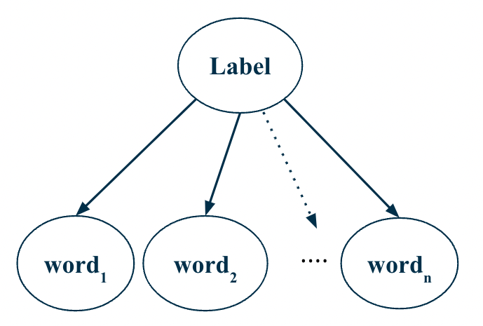
Naive Bayes’ makes a simplifying naive assumption that the features are independent of each other, given the class. In other words,
\[ P(X|y) = \prod_{i=1}^{D} P(x_i|y) \]

This is a naive assumption, since in most cases, features are not independent. This is especially not true for text data, where the presence of a word in a document is highly correlated with the presence of other words in the document. Hence the popular adage in NLP: “You shall know a word by the company it keeps” by Firth.
However, the naive assumption makes the computation of the likelihood term tractable and still remarkably yields great results in practice.
Naive Bayes model is a generative model since it makes an assumption about how the data is generated. It assumes that the data is generated by first sampling a class \(y\) from the prior distribution \(P(y)\) and then sampling each feature \(x_i\) from the likelihood distribution \(P(x_i|y)\).
Bag of Words (BOW) as Multinomial Data
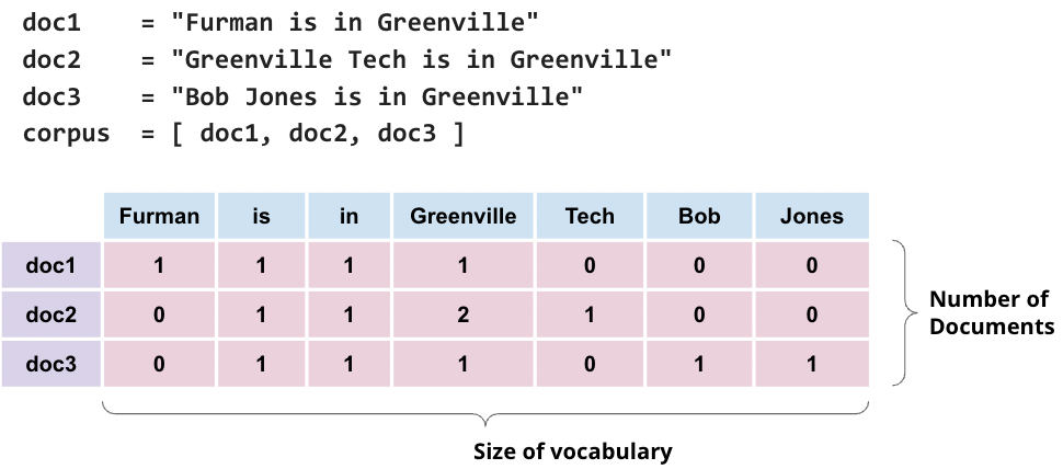
Recall that multinomial distribution counts the number of times an outcome occurs when there are k-possible outcomes and N independent trials that can be used to capture probability of counts for rolling a k-sided die n times. Also recall that BOW representation of text is a count of how many times a word occurs in a document.
BOW representation, therefore, can be modeled using the multinomial distibution. Here, instead of k-sided die, imagine a \(|V|\) sided die where \(V\) is the set of all unique words (vocabulary) and \(|V|\) is the size of the vocabulary. Each word in the vocabulary, in other words, is a possible outcome and count of a word in all documents constitutes a binomial distribution of that word.


So we can use the multinomial distribution to model the likelihood term \(P(x_i|y)\) in the prediction rule.
However, the Naive Assumption in the Naive Bayes model alleviates the need to estimate the joint distribution of the features. Instead, we can estimate the parameters of the binomial distribution for each feature independently and simply multiply the probabilities of each feature to get the likelihood term.
The parameters of the binomial distribution are estimated using Maximum Likelihood Estimation (MLE) or Maximum A Posteriori (MAP) estimation.
Multinomial Naive Bayes Classifier
Naive Bayes classifier is simply a probabilistic classifier where the prediction \(\hat{y}\) is the class \(y\) that maximizes the posterior probability \(P(\mathbf{y}|X)\) i.e.
\[ \hat{y} = \underset{y}{\operatorname{argmax}} P(\mathbf{y}|X) \]
In other words, if y=0 maximizes P(y | X), then the predicted class is 0. Otherwise, if y=1 maximizes P(y | X), then the predicted class is 1.
P(y | X) is proportional to P(X | y)P(y), as per the Bayes’ theorem. In other words, we can ignore the denominator P(X) since it is the same for all classes (values of \(\textbf{y}\)).
So, we can also write the prediction rule as:
\[ \hat{y} = \underset{y}{\operatorname{argmax}} P(X|\mathbf{y})\cdot P(\mathbf{y}) \]
If we make the naive assumption that the features are independent of each other, given the class, then we can write the prediction rule as:
\[ \hat{y} = \underset{y}{\operatorname{argmax}} \prod_{i=1}^{D} P(x_i|\mathbf{y}) \cdot P(\mathbf{y}) \]
Based on our conversation on logarithms, when we apply log to the equation above, two things happen:
Due to log being a monotonically increasing function, the outcome of argmax remains unchanged.
All multiplications in the equation become additions, making our lives easier.
Therefore, we can write the prediction rule as:
\[ \hat{y} = \underset{y}{\operatorname{argmax}} \sum_{i=1}^{D} \log P(x_i|\mathbf{y}) + \log P(\mathbf{y}) \]
Now, let’s look at the two terms in the equation above:
\(P(\mathbf{y})\) is the prior probability of the class \(y\). It is estimated as the fraction of documents in the training set that belong to class \(y\).
\(P(x_i|\mathbf{y})\) is the likelihood term. It is the sum of the log probabilities of each \(x_i\) \(X\) given the class \(y\).
If, for example, we are trying to predict the sentiment of the document “Furman University” then the likelihood term would be \(\text{log}~ P(\text{Furman}|y) + \text{log}~ P(\text{University}|y)\).
Similarly, likelihood term for the document “Greeenville is in SC” would be \(\text{log}~P(\text{Greenville}|y) + \text{log}~ P(\text{is}|y) + \text{log}~ P(\text{in}|y) + \text{log}~ P(\text{SC}|y)\).