Machine learning models require clean and well-structured data to perform effectively.
Two common techniques for preparing data are normalization and standardization.
Normalization scales the data to a fixed range, typically [0, 1], while standardization transforms the data to have a mean of 0 and a standard deviation of 1.
import pandas as pd url ="https://raw.githubusercontent.com/fahadsultan/csc272/main/data/elections.csv"elections = pd.read_csv(url)elections.head()
Year
Candidate
Party
Popular vote
Result
%
0
1824
Andrew Jackson
Democratic-Republican
151271
loss
57.210122
1
1824
John Quincy Adams
Democratic-Republican
113142
win
42.789878
2
1828
Andrew Jackson
Democratic
642806
win
56.203927
3
1828
John Quincy Adams
National Republican
500897
loss
43.796073
4
1832
Andrew Jackson
Democratic
702735
win
54.574789
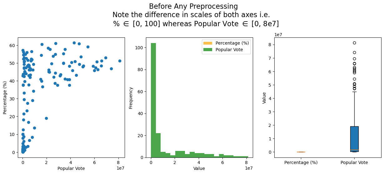
from matplotlib import pyplot as plt fig, axs = plt.subplots(1, 3, figsize=(15, 5))axs[0].scatter(elections['Popular vote'], elections['%']);axs[0].set_xlabel('Popular Vote');axs[0].set_ylabel('Percentage (%)');# axs[0].set_title('');axs[1].hist(elections['%'], bins=20, color='orange', alpha=0.7, label='Percentage (%)');axs[1].hist(elections['Popular vote'], bins=20, color='green', alpha=0.7, label='Popular Vote');axs[1].set_xlabel('Value');axs[1].set_ylabel('Frequency');# axs[1].set_title('Note the difference in distributions of both features');axs[1].legend();axs[2].boxplot([elections['%'], elections['Popular vote']], vert=True, patch_artist=True, labels=['Percentage (%)', 'Popular Vote']);axs[2].set_ylabel('Value');# axs[2].set_title('Note the difference in scales of both features');fig.suptitle('Before Any Preprocessing\nNote the difference in scales of both axes i.e. \n % $\in$ [0, 100] whereas Popular Vote $\in$ [0, 8e7]', fontsize=16, y=1.1);
Min-Max Normalization
Feature scaling is a technique used to standardize the range of independent variables or features of data.
For instance, consider a dataset with two features: age (ranging from 0 to 100) and income (ranging from 0 to 1,000,000).
If we do not scale these features, a machine learning algorithm may give disproportionate attention to the income feature due to its larger range.
In order to address this issue, we can apply normalization techniques such as Min-Max Normalization.
Min-Max Normalization scales the data to a fixed range, usually [0, 1]. The formula for Min-Max Normalization is:
\(\text{min}(X)\) is the minimum value (scalar) of the \(X\).
\(\text{max}(X)\) is also the maximum value (scalar) of the \(X\).
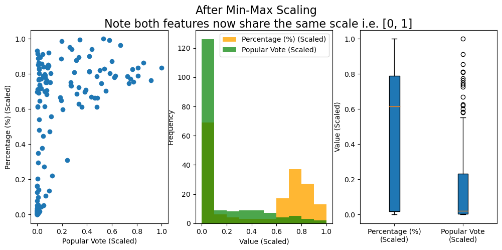
# Import MinMax scalerfrom sklearn.preprocessing import MinMaxScalerfig, axs = plt.subplots(1, 3, figsize=(12, 5))# Create a MinMaxScaler objectscaler = MinMaxScaler()# Fit and transform the 'total_votes' columnelections['Popular vote scaled'] = scaler.fit_transform(elections[['Popular vote']])elections['% scaled'] = scaler.fit_transform(elections[['%']])# Display the first few rows of the updated DataFrameaxs[0].scatter(elections['Popular vote scaled'], elections['% scaled']);axs[0].set_xlabel('Popular Vote (Scaled)');axs[0].set_ylabel('Percentage (%) (Scaled)');# axs[0].set_title('After Min-Max Scaling\n\n Note both axes now share the same scale i.e. \n % $\in$ [0, 1] and Popular Vote $\in$ [0, 1]');axs[1].hist(elections['% scaled'], bins=10, color='orange', alpha=0.8, label='Percentage (%) (Scaled)');axs[1].hist(elections['Popular vote scaled'], bins=10, color='green', alpha=0.7, label='Popular Vote (Scaled)');axs[1].set_xlabel('Value (Scaled)');axs[1].set_ylabel('Frequency');axs[1].legend();axs[2].boxplot([elections['% scaled'], elections['Popular vote scaled']], vert=True, patch_artist=True, labels=['Percentage (%)\n(Scaled)', 'Popular Vote\n(Scaled)']);axs[2].set_ylabel('Value (Scaled)');fig.suptitle('After Min-Max Scaling\n Note both features now share the same scale i.e. [0, 1]', fontsize=16);
Z-Scores Standardization
Commonly used in machine learning, standardization transforms the data to have a mean of 0 and a standard deviation of 1.
The formula for Z-Score Standardization is:
\[ Z = \frac{X - \mu}{\sigma} \]
Where:
\(X\) is the original column vector.
\(Z\) is the standardized column vector.
\(\mu\) is the mean of the feature.
\(\sigma\) is the standard deviation of the feature.
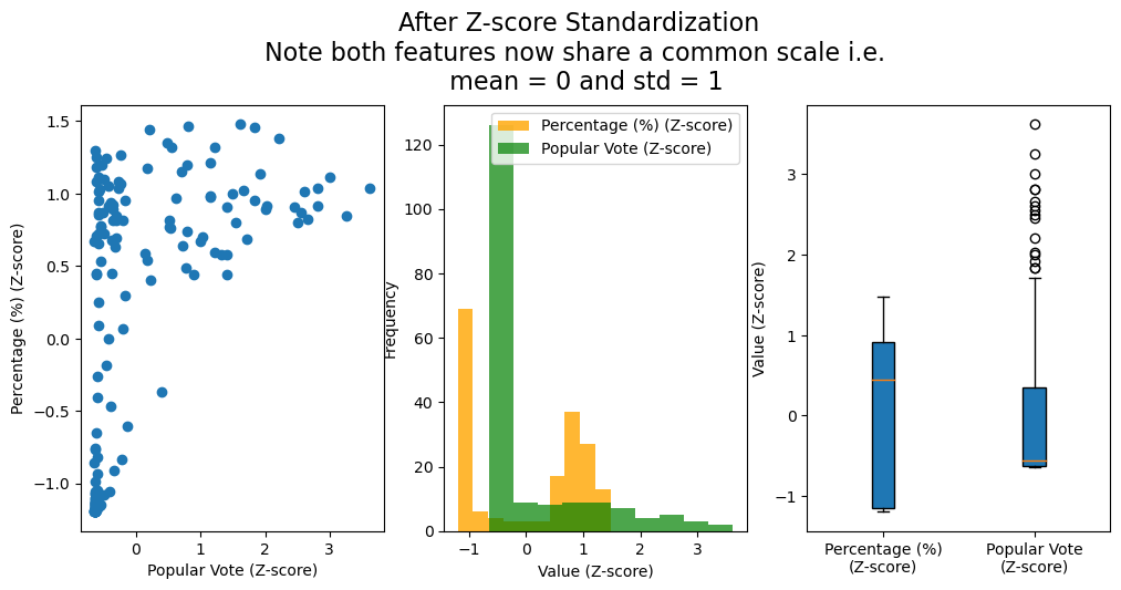
#import z-score from sklearn.preprocessing import StandardScalerfig, axs = plt.subplots(1, 3, figsize=(12, 5))# Create a StandardScaler objectscaler = StandardScaler()# Fit and transform the 'total_votes' columnelections['Popular vote zscore'] = scaler.fit_transform(elections[['Popular vote']])elections['% zscore'] = scaler.fit_transform(elections[['%']])# Display the first few rows of the updated DataFrameaxs[0].scatter(elections['Popular vote zscore'], elections['% zscore']);axs[0].set_xlabel('Popular Vote (Z-score)');axs[0].set_ylabel('Percentage (%) (Z-score)');# axs[0].set_title('Note both axes now share a common scale i.e. \n mean = 0 and std = 1');axs[1].hist(elections['% zscore'], bins=10, color='orange', alpha=0.8, label='Percentage (%) (Z-score)');axs[1].hist(elections['Popular vote zscore'], bins=10, color='green', alpha=0.7, label='Popular Vote (Z-score)');axs[1].set_xlabel('Value (Z-score)');axs[1].set_ylabel('Frequency');axs[1].set_title('');axs[1].legend();axs[2].boxplot([elections['% zscore'], elections['Popular vote zscore']], vert=True, patch_artist=True, labels=['Percentage (%)\n(Z-score)', 'Popular Vote\n(Z-score)']);axs[2].set_ylabel('Value (Z-score)');fig.suptitle('After Z-score Standardization\n Note both features now share a common scale i.e. \n mean = 0 and std = 1', fontsize=16, y=1.05);
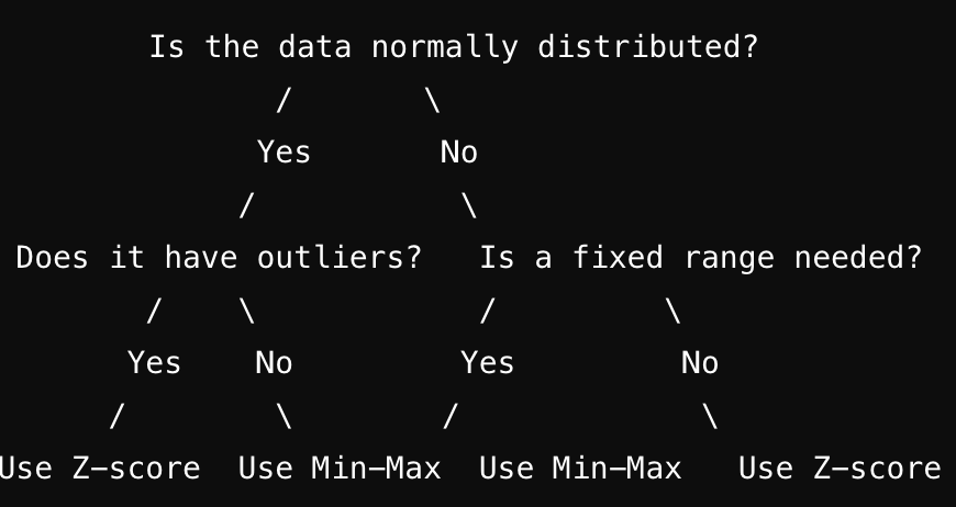
When Should You Use Each Technique?
Use Min-Max Normalization when the data does not follow a Gaussian distribution (bell curve) and when you want to bound the values within a specific range.
Note that if you have extreme outliers in your data, Min-Max Normalization will not be effective, as the outliers will skew the min and max values, leading to a compressed range for the majority of the data points.
Use Z-Score Standardization when the data follows a Gaussian distribution (bell curve) or when you want to center the data around the mean with a standard deviation of 1.
When your data contains outliers, Z-Score Standardization is generally more robust than Min-Max Normalization, as it focuses on the mean and standard deviation rather than the extreme values.