Model Selection

Model selection is a critical step in the machine learning workflow that involves choosing the best model from a set of candidate models based on their performance on a given dataset. The goal is to select a model that generalizes well to unseen data, rather than just performing well on the training data.

Model selection generally only applies to supervised learning tasks, where the dataset consists of input-output pairs.

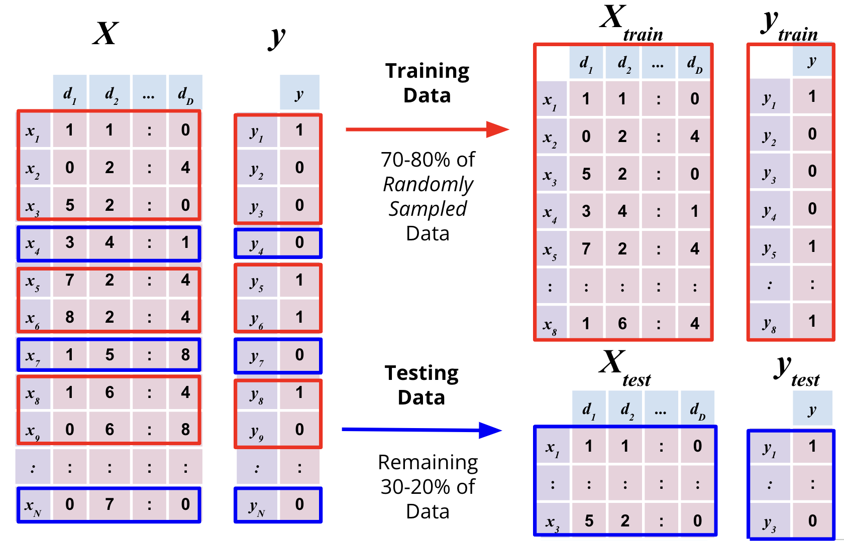
Training and Test Sets

For effective model validation, the dataset is typically divided into atleast two subsets:

1. Training Set: This subset is used to train the model. Training involves feeding the model with input data and corresponding labels so that it can learn patterns and relationships.

2. Test Set: This subset is used to assess the final performance of the model after training and validation. It provides an unbiased evaluation of the model’s generalization ability. It is extremely important that the test set remains completely unseen during the training to ensure an unbiased evaluation of the model’s performance.

In some cases, a third subset called the Validation Set is also used during the training process to tune hyperparameters and make decisions about model architecture. However, in simpler workflows, cross-validation techniques can be employed instead of a separate validation set.

In sklearn, the train_test_split function from the model_selection module is commonly used to split the dataset into training and test sets. Here is an example:

import pandas as pd 
from sklearn.model_selection import train_test_split

url = "https://raw.githubusercontent.com/fahadsultan/csc272/main/data/elections.csv"

elections = pd.read_csv(url)

elections.head()

	Year	Candidate	Party	Popular vote	Result	%
0	1824	Andrew Jackson	Democratic-Republican	151271	loss	57.210122
1	1824	John Quincy Adams	Democratic-Republican	113142	win	42.789878
2	1828	Andrew Jackson	Democratic	642806	win	56.203927
3	1828	John Quincy Adams	National Republican	500897	loss	43.796073
4	1832	Andrew Jackson	Democratic	702735	win	54.574789

X = elections[['Year', 'Popular vote']]

y = elections['Result']

X_train, X_test, y_train, y_test = train_test_split(X, y, test_size=0.3, random_state=42)

X_train.shape, y_train.shape

((127, 2), (127,))

X_test.shape, y_test.shape

((55, 2), (55,))

Performance Metrics

Depending on the type of problem (classification, regression, etc.), different metrics are used to evaluate model performance. Common metrics include accuracy, precision, recall, F1-score for classification tasks, and mean squared error (MSE), R-squared for regression tasks.

Classification Metrics

The most common metric for evaluating a classifier is accuracy. Accuracy is the proportion of correct predictions. It is the number of correct predictions divided by the total number of predictions.

\[Accuracy = \frac{\text{Number of correct predictions}}{\text{Total number of predictions}}\]

For example, if we have a test set of 100 documents, and our classifier correctly predicts the class of 80 of them, then the accuracy is 80%.

Accuracy is a good metric when the classes are balanced \(N_{class1} \approx N_{class2}\). However, when the classes are imbalanced, accuracy can be misleading. For example, if we have a test set of 100 documents, and 95 of them are positive and 5 of them are negative, then a classifier that always predicts positive will have an accuracy of 95%. However, this classifier is not useful, because it never predicts negative.

Multi-class classification as multiple Binary classifications

Every multi-class classification problem can be decomposed into multiple binary classification problems. For example, if we have a multi-class classification problem with 3 classes, we can decompose it into 3 binary classification problems.

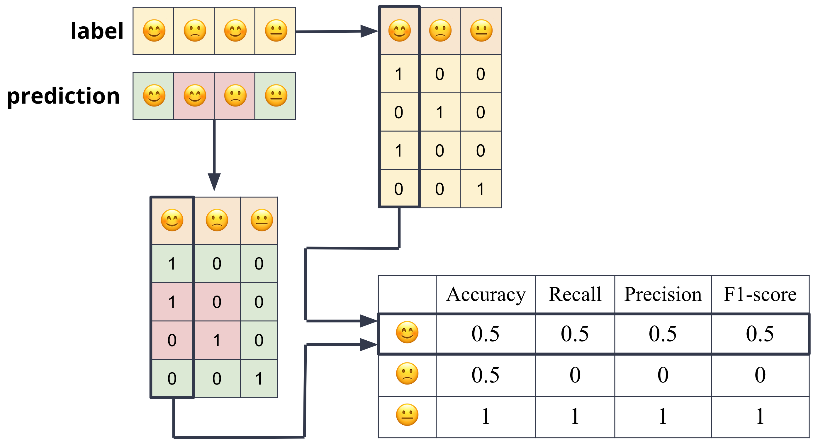
Assuming the categorical variable that we are trying to predict is binary, we can define the accuracy in terms of the four possible outcomes of a binary classifier:

1. True Positive (TP): The classifier correctly predicted the positive class.
2. False Positive (FP): The classifier incorrectly predicted the negative class as positive.
3. True Negative (TN): The classifier correctly predicted the negative class.
4. False Negative (FN): The classifier incorrectly predicted the positive class as negative.

True positive means that the classifier correctly predicted the positive class. False positive means that the classifier incorrectly predicted the positive class. True negative means that the classifier correctly predicted the negative class. False negative means that the classifier incorrectly predicted the negative class.

These definitions are summarized in the table below:

	Prediction \(\hat{y} = f'(x)\)	Truth \(y = f(x)\)
True Negative (TN)	0	0
False Negative (FN)	0	1
False Positive (FP)	1	0
True Positive (TP)	1	1

In terms of the four outcomes above, the accuracy is:

\[ \text{Accuracy} = \frac{TP + TN}{TP + TN + FP + FN}\]

Accuracy is a useful metric, but it can be misleading.

Other metrics that are often used to evaluate classifiers are:

• Precision: The proportion of positive predictions that are correct. Mathematically, it is defined as:

\[\text{Precision} = \frac{TP}{TP + FP}\]

• Recall: The proportion of positive instances that are correctly predicted. Mathematically, it is defined as:

\[\text{Recall} = \frac{TP}{TP + FN}\]

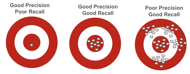
Intuitively, precision measures how many of the predicted positive instances are actually positive, while recall measures how many of the actual positive instances are correctly predicted.

For example, consider a binary classification problem where we have 100 actual positive instances and 100 actual negative instances.

If the model predicts 10 positive instances, of which 9 are correct (true positives) and 1 is incorrect (false positive), then the precision is 0.9 (9/10) and the recall is 0.09 (9/100).

A model with perfect precision but poor recall predicts positives only when it’s absolutely certain, so it never makes a false positive, but it misses most true positives—for example, predicting only 5 correct positives out of 100 actual positives (precision = 1.0, recall = 0.05).

In contrast, a model with poor precision but good recall predicts many more positives than truly exist, catching almost all real positives but generating many false alarms—for instance, predicting 200 positives when only 90 are correct out of 100 actual positives (precision = 0.45, recall = 0.90).

The precision and recall are often combined into a single metric called the F1 score. The F1 score is the harmonic mean of precision and recall. The harmonic mean of two numbers is given by:

• F1 Score: The harmonic mean of precision and recall.

\[\text{F1-Score} = 2 \times \frac{\text{Precision} \cdot \text{Recall}}{\text{Precision} + \text{Recall}}\]

from sklearn.model_selection import train_test_split
from sklearn.metrics import accuracy_score, mean_squared_error, r2_score
from sklearn.dummy import DummyClassifier, DummyRegressor

X = elections[['Year', 'Popular vote']]
y = elections['Result']

model = DummyClassifier(strategy='most_frequent')

# Example for classification
X_train, X_test, y_train, y_test = train_test_split(X, y, test_size=0.2, random_state=42)
model.fit(X_train, y_train)
y_pred = model.predict(X_test)
accuracy = accuracy_score(y_test, y_pred)
print(f'Accuracy: {accuracy}')

In sklearn, various performance metrics can be computed using functions from the metrics module. Here is an example of how to compute accuracy, precision, recall, and F1-score:

from sklearn.metrics import accuracy_score, precision_score, recall_score, f1_score
y_true = [0, 1, 1, 0, 1]
y_pred = [0, 1, 0, 0, 1]

accuracy = accuracy_score(y_true, y_pred)
precision = precision_score(y_true, y_pred)
recall = recall_score(y_true, y_pred)
f1 = f1_score(y_true, y_pred)
print(f'Accuracy: {accuracy}')
print(f'Precision: {precision}')
print(f'Recall: {recall}')
print(f'F1 Score: {f1}')

Accuracy: 0.8
Precision: 1.0
Recall: 0.6666666666666666
F1 Score: 0.8

In this example, y_true represents the true labels, and y_pred represents the predicted labels from the model. The functions compute the respective metrics based on these labels.

sklearn also provides a classification_report function that summarizes multiple metrics in a single report:

from sklearn.metrics import classification_report
y_true = [0, 1, 1, 0, 1]
y_pred = [0, 1, 0, 0, 1]
report = classification_report(y_true, y_pred, target_names=['Class 0', 'Class 1'])
print(report)

              precision    recall  f1-score   support

     Class 0       0.67      1.00      0.80         2
     Class 1       1.00      0.67      0.80         3

    accuracy                           0.80         5
   macro avg       0.83      0.83      0.80         5
weighted avg       0.87      0.80      0.80         5

Regression Metrics

For regression tasks, common performance metrics include:

• Mean Absolute Error (MAE): The average of the absolute differences between the predicted and actual values.

\[\text{MAE} = \frac{1}{n} \sum_{i=1}^{n} |y_i - \hat{y}_i|\]

• Mean Squared Error (MSE): The average of the squared differences between the predicted and actual values.

\[\text{MSE} = \frac{1}{n} \sum_{i=1}^{n} (y_i - \hat{y}_i)^2\]

• R-squared (R²): A statistical measure that represents the proportion of the variance for a dependent variable that’s explained by an independent variable or variables in a regression model.

\[R^2 = 1 - \frac{\sum_{i=1}^{n} (y_i - \hat{y}_i)^2}{\sum_{i=1}^{n} (y_i - \bar{y})^2}\]

Where:

• \(y_i\) is the actual value
• \(\hat{y}_i\) is the predicted value
• \(\bar{y}\) is the mean of the actual values

from sklearn.model_selection import train_test_split
from sklearn.metrics import accuracy_score, mean_squared_error, r2_score

X = elections[['Year', 'Popular vote']]
y = elections['Result']

# Example for regression
X_train, X_test, y_train, y_test = train_test_split(X, y, test_size=0.2, random_state=42)
model.fit(X_train, y_train)
y_pred = model.predict(X_test)
mse = mean_squared_error(y_test, y_pred)
r2 = r2_score(y_test, y_pred)
print(f'Mean Squared Error: {mse}')
print(f'R-squared: {r2}')

Baseline Models

Establishing a baseline is an essential step in model validation. A baseline provides a reference point against which the performance of more complex models can be compared. It helps to determine whether a new model is actually improving upon simpler approaches.

In sklearn, you can easily implement these baseline models using DummyClassifier for classification tasks and DummyRegressor for regression tasks to create baseline models.

Random Baseline

A model that makes random predictions. This is often used to demonstrate that a more sophisticated model performs better than chance.

In case of DummyClassifier and DummyRegressor, you can set the strategy to “uniform” to achieve this.

random_predictor = DummyClassifier(strategy="uniform")
random_regressor = DummyRegressor(strategy="uniform")

Majority Class Baseline

In classification tasks, this baseline predicts the most frequent class in the training data for all instances. This is particularly useful in imbalanced datasets.

In case of DummyClassifier, you can set the strategy to “most_frequent” to achieve this. DummyRegressor does not have a direct equivalent for majority class, but you can use the mean strategy for regression tasks.

majority_class_predictor = DummyClassifier(strategy="most_frequent")

Mean/Median Baseline

For regression tasks, a common baseline is to predict the mean or median of the target variable. This provides a simple benchmark for evaluating the performance of regression models.

mean_regressor = DummyRegressor(strategy="mean")
median_regressor = DummyRegressor(strategy="median")

These baseline models can be trained and evaluated in the same way as any other model in sklearn, allowing for straightforward comparisons of performance.

from sklearn.dummy import DummyClassifier, DummyRegressor
from sklearn.model_selection import train_test_split
from sklearn.metrics import accuracy_score, mean_squared_error

# Example for classification
X_train, X_test, y_train, y_test = train_test_split(X, y, test_size=0.2, random_state=42)
dummy_clf = DummyClassifier(strategy="most_frequent")
dummy_clf.fit(X_train, y_train)
y_pred = dummy_clf.predict(X_test)
print("Baseline Accuracy:", accuracy_score(y_test, y_pred))

# Example for regression
dummy_reg = DummyRegressor(strategy="mean")
dummy_reg.fit(X_train, y_train)
y_pred = dummy_reg.predict(X_test)
print("Baseline MSE:", mean_squared_error(y_test, y_pred))

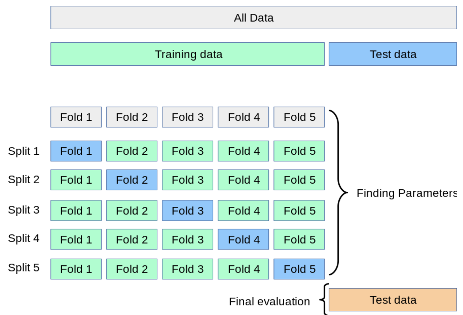
Cross-Validation

• A technique used to assess how the results of a statistical analysis will generalize to an independent dataset. Common methods include k-fold cross-validation and leave-one-out cross-validation.

k-fold cross-validation involves dividing the dataset into k subsets (or “folds”).

The model is trained on k-1 folds and validated on the remaining fold.

This process is repeated k times, with each fold serving as the validation set once.

The final performance metric is typically the average of the metrics obtained from each fold.

# cross validation
from sklearn.model_selection import cross_val_score
from sklearn.neighbors import KNeighborsClassifier

knn = KNeighborsClassifier(n_neighbors=5)
scores = cross_val_score(knn, X, y, cv=5)
scores.mean()
scores.std()
scores
knn.fit(X_train, y_train)
knn.score(X_test, y_test)
y_pred = knn.predict(X_test)
from sklearn.metrics import classification_report, confusion_matrix
print(confusion_matrix(y_test, y_pred))
print(classification_report(y_test, y_pred))

Overfitting and Underfitting

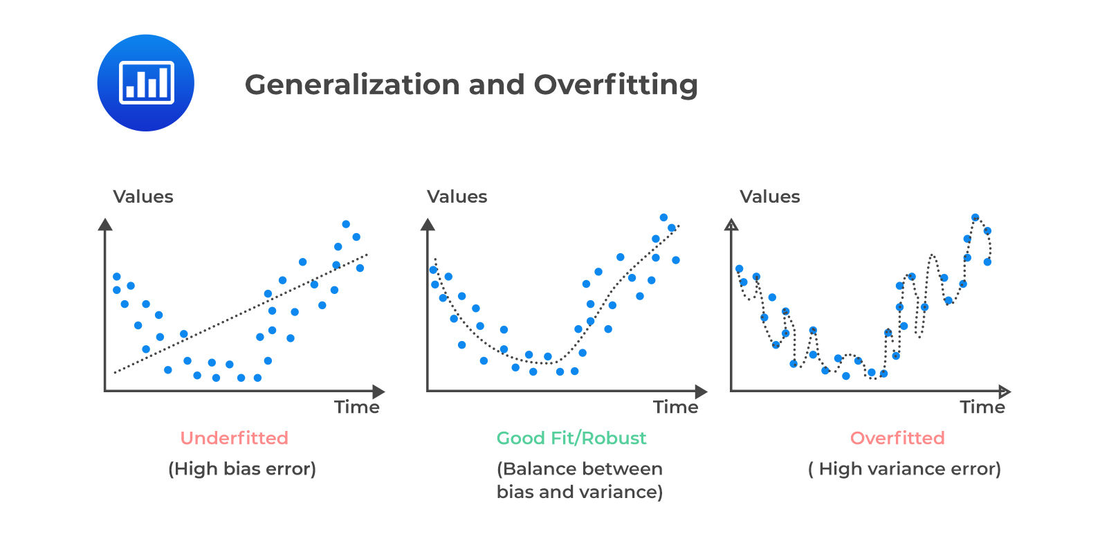
The overarching goal of model selection is to find a model that generalizes well to unseen data. Two common pitfalls in this process are overfitting and underfitting:

• Overfitting: When a model learns the training data too well, including noise and outliers, leading to poor generalization on new data.

This often occurs when the model is too complex relative to the amount of training data available. Overfitting can be detected when the model performs significantly better on the training set compared to the test set.

• Underfitting: When a model is too simple to capture the underlying patterns in the data, resulting in poor performance on both training and test sets.

Underfitting can be identified when the model performs poorly on both the training and test sets, indicating that it has not learned the data well enough.