names.head()| Name | Sex | Count | Year | First Letter | |
|---|---|---|---|---|---|
| 0 | Mary | F | 7065 | 1880 | M |
| 1 | Anna | F | 2604 | 1880 | A |
| 2 | Emma | F | 2003 | 1880 | E |
| 3 | Elizabeth | F | 1939 | 1880 | E |
| 4 | Minnie | F | 1746 | 1880 | M |
We know now that .groupby gives us the ability to group and aggregate data across our DataFrame. The examples above formed groups using just one column in the DataFrame. It’s possible to group by multiple columns at once by passing in a list of column names to .groupby.
Let’s consider the names dataset. In this problem, we will find the total number of baby names associated with each sex for each year. To do this, we’ll group by both the "Year" and "Sex" columns.
| Name | Sex | Count | Year | First Letter | |
|---|---|---|---|---|---|
| 0 | Mary | F | 7065 | 1880 | M |
| 1 | Anna | F | 2604 | 1880 | A |
| 2 | Emma | F | 2003 | 1880 | E |
| 3 | Elizabeth | F | 1939 | 1880 | E |
| 4 | Minnie | F | 1746 | 1880 | M |
# Find the total number of baby names associated with each sex for each year in the data
names.groupby(["Year", "Sex"])[["Count"]].sum().head(6)| Count | ||
|---|---|---|
| Year | Sex | |
| 1880 | F | 90994 |
| M | 110490 | |
| 1881 | F | 91953 |
| M | 100737 | |
| 1882 | F | 107847 |
| M | 113686 |
Notice that both "Year" and "Sex" serve as the index of the DataFrame (they are both rendered in bold). We’ve created a multi-index DataFrame where two different index values, the year and sex, are used to uniquely identify each row.
This isn’t the most intuitive way of representing this data – and, because multi-indexed DataFrames have multiple dimensions in their index, they can often be difficult to use.
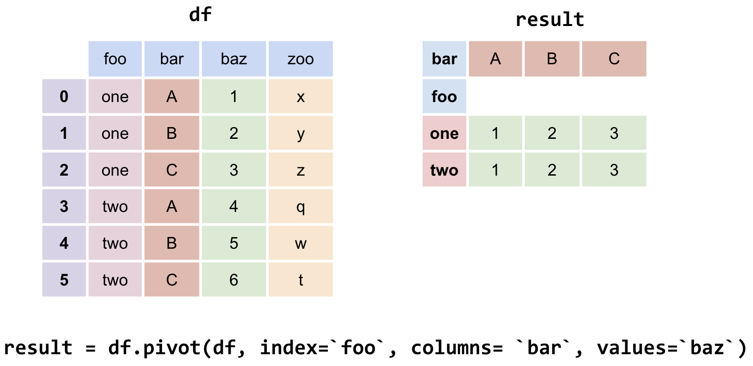
Another strategy to aggregate across two columns is to create a pivot table. One set of values is used to create the index of the pivot table; another set is used to define the column names. The values contained in each cell of the table correspond to the aggregated data for each index-column pair.
The best way to understand pivot tables is to see one in action. Let’s return to our original goal of summing the total number of names associated with each combination of year and sex. We’ll call the pandas .pivot_table method to create a new table.
# The `pivot_table` method is used to generate a Pandas pivot table
names.pivot_table(
    index = "Year",
    columns = "Sex",
    values = "Count",
aggfunc = sum).head(5)| Sex | F | M |
|---|---|---|
| Year | ||
| 1880 | 90994 | 110490 |
| 1881 | 91953 | 100737 |
| 1882 | 107847 | 113686 |
| 1883 | 112319 | 104625 |
| 1884 | 129019 | 114442 |
Looks a lot better! Now, our DataFrame is structured with clear index-column combinations. Each entry in the pivot table represents the summed count of names for a given combination of "Year" and "Sex".
Let’s take a closer look at the code implemented above.
index = "Year" specifies the column name in the original DataFrame that should be used as the index of the pivot tablecolumns = "Sex" specifies the column name in the original DataFrame that should be used to generate the columns of the pivot tablevalues = "Count" indicates what values from the original DataFrame should be used to populate the entry for each index-column combinationaggfunc = sum tells pandas what function to use when aggregating the data specified by values. Here, we are summing the name counts for each pair of "Year" and "Sex"
We can even include multiple values in the index or columns of our pivot tables.
names_pivot = names.pivot_table(
    index="Year",     # the rows (turned into index)
    columns="Sex",    # the column values
    values=["Count", "Name"],
    aggfunc=max,   # group operation
)
names_pivot.head(6)| Count | Name | |||
|---|---|---|---|---|
| Sex | F | M | F | M |
| Year | ||||
| 1880 | 7065 | 9655 | Zula | Zeke |
| 1881 | 6919 | 8769 | Zula | Zeb |
| 1882 | 8148 | 9557 | Zula | Zed |
| 1883 | 8012 | 8894 | Zula | Zeno |
| 1884 | 9217 | 9388 | Zula | Zollie |
| 1885 | 9128 | 8756 | Zula | Zollie |