In this section, we will learn how to use representations of audio data in machine learning.
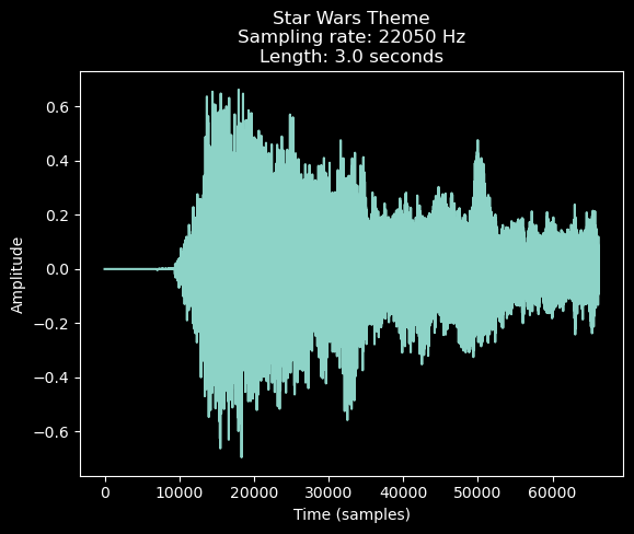
Audio files can be represented in a variety of ways. The most common is the waveform , which is a time series of the amplitude of the sound wave at each time point. The waveform is a one-dimensional array of numbers. The sampling rate is the number of samples per second.
To load an audio file, we can use the librosa library. The librosa.load function returns the waveform and the sampling rate.
You may have to install the librosa library using !pip install librosa in a new code cell for the code below to work.
The audio file can be downloaded from this link .
Requirement already satisfied: librosa in /Users/fsultan/opt/anaconda3/lib/python3.9/site-packages (0.10.1)
Requirement already satisfied: audioread>=2.1.9 in /Users/fsultan/opt/anaconda3/lib/python3.9/site-packages (from librosa) (3.0.0)
Requirement already satisfied: numpy!=1.22.0,!=1.22.1,!=1.22.2,>=1.20.3 in /Users/fsultan/opt/anaconda3/lib/python3.9/site-packages (from librosa) (2.0.2)
Requirement already satisfied: scipy>=1.2.0 in /Users/fsultan/opt/anaconda3/lib/python3.9/site-packages (from librosa) (1.13.1)
Requirement already satisfied: scikit-learn>=0.20.0 in /Users/fsultan/opt/anaconda3/lib/python3.9/site-packages (from librosa) (1.0.2)
Requirement already satisfied: joblib>=0.14 in /Users/fsultan/opt/anaconda3/lib/python3.9/site-packages (from librosa) (1.1.0)
Requirement already satisfied: decorator>=4.3.0 in /Users/fsultan/opt/anaconda3/lib/python3.9/site-packages (from librosa) (5.1.1)
Requirement already satisfied: numba>=0.51.0 in /Users/fsultan/opt/anaconda3/lib/python3.9/site-packages (from librosa) (0.55.1)
Requirement already satisfied: soundfile>=0.12.1 in /Users/fsultan/opt/anaconda3/lib/python3.9/site-packages (from librosa) (0.12.1)
Requirement already satisfied: pooch>=1.0 in /Users/fsultan/opt/anaconda3/lib/python3.9/site-packages (from librosa) (1.7.0)
Requirement already satisfied: soxr>=0.3.2 in /Users/fsultan/opt/anaconda3/lib/python3.9/site-packages (from librosa) (0.3.6)
Requirement already satisfied: typing-extensions>=4.1.1 in /Users/fsultan/opt/anaconda3/lib/python3.9/site-packages (from librosa) (4.12.2)
Requirement already satisfied: lazy-loader>=0.1 in /Users/fsultan/opt/anaconda3/lib/python3.9/site-packages (from librosa) (0.3)
Requirement already satisfied: msgpack>=1.0 in /Users/fsultan/opt/anaconda3/lib/python3.9/site-packages (from librosa) (1.0.2)
Requirement already satisfied: llvmlite<0.39,>=0.38.0rc1 in /Users/fsultan/opt/anaconda3/lib/python3.9/site-packages (from numba>=0.51.0->librosa) (0.38.0)
Collecting numpy!=1.22.0,!=1.22.1,!=1.22.2,>=1.20.3 (from librosa)
  Downloading numpy-1.21.6-cp39-cp39-macosx_10_9_x86_64.whl.metadata (2.1 kB)
Requirement already satisfied: setuptools in /Users/fsultan/opt/anaconda3/lib/python3.9/site-packages (from numba>=0.51.0->librosa) (73.0.1)
Requirement already satisfied: platformdirs>=2.5.0 in /Users/fsultan/opt/anaconda3/lib/python3.9/site-packages (from pooch>=1.0->librosa) (4.2.2)
Requirement already satisfied: packaging>=20.0 in /Users/fsultan/opt/anaconda3/lib/python3.9/site-packages (from pooch>=1.0->librosa) (24.1)
Requirement already satisfied: requests>=2.19.0 in /Users/fsultan/opt/anaconda3/lib/python3.9/site-packages (from pooch>=1.0->librosa) (2.32.3)
Requirement already satisfied: threadpoolctl>=2.0.0 in /Users/fsultan/opt/anaconda3/lib/python3.9/site-packages (from scikit-learn>=0.20.0->librosa) (2.2.0)
INFO: pip is looking at multiple versions of scipy to determine which version is compatible with other requirements. This could take a while.
Collecting scipy>=1.2.0 (from librosa)
  Downloading scipy-1.13.0-cp39-cp39-macosx_10_9_x86_64.whl.metadata (60 kB)
  Downloading scipy-1.12.0-cp39-cp39-macosx_10_9_x86_64.whl.metadata (60 kB)
  Downloading scipy-1.11.4-cp39-cp39-macosx_10_9_x86_64.whl.metadata (60 kB)
Requirement already satisfied: cffi>=1.0 in /Users/fsultan/opt/anaconda3/lib/python3.9/site-packages (from soundfile>=0.12.1->librosa) (1.15.0)
Requirement already satisfied: pycparser in /Users/fsultan/opt/anaconda3/lib/python3.9/site-packages (from cffi>=1.0->soundfile>=0.12.1->librosa) (2.21)
Requirement already satisfied: charset-normalizer<4,>=2 in /Users/fsultan/opt/anaconda3/lib/python3.9/site-packages (from requests>=2.19.0->pooch>=1.0->librosa) (3.3.2)
Requirement already satisfied: idna<4,>=2.5 in /Users/fsultan/opt/anaconda3/lib/python3.9/site-packages (from requests>=2.19.0->pooch>=1.0->librosa) (3.8)
Requirement already satisfied: urllib3<3,>=1.21.1 in /Users/fsultan/opt/anaconda3/lib/python3.9/site-packages (from requests>=2.19.0->pooch>=1.0->librosa) (2.2.2)
Requirement already satisfied: certifi>=2017.4.17 in /Users/fsultan/opt/anaconda3/lib/python3.9/site-packages (from requests>=2.19.0->pooch>=1.0->librosa) (2024.7.4)
Downloading numpy-1.21.6-cp39-cp39-macosx_10_9_x86_64.whl (17.0 MB)
   ━━━━━━━━━━━━━━━━━━━━━━━━━━━━━━━━━━━━━━━━ 17.0/17.0 MB 7.9 MB/s eta 0:00:00a 0:00:01
Downloading scipy-1.11.4-cp39-cp39-macosx_10_9_x86_64.whl (37.3 MB)
   ━━━━━━━━━━━━━━━━━━━━━━━━━━━━━━━━━━━━━━━━ 37.3/37.3 MB 18.7 MB/s eta 0:00:00a 0:00:01
Installing collected packages: numpy, scipy
  Attempting uninstall: numpy
    Found existing installation: numpy 2.0.2
    Uninstalling numpy-2.0.2:
      Successfully uninstalled numpy-2.0.2
  Attempting uninstall: scipy
    Found existing installation: scipy 1.13.1
    Uninstalling scipy-1.13.1:
      Successfully uninstalled scipy-1.13.1
ERROR: pip's dependency resolver does not currently take into account all the packages that are installed. This behaviour is the source of the following dependency conflicts.
daal4py 2021.5.0 requires daal==2021.4.0, which is not installed.
nibabel 5.3.2 requires numpy>=1.22, but you have numpy 1.21.6 which is incompatible.
panel 0.13.0 requires bokeh<2.5.0,>=2.4.0, but you have bokeh 3.2.0 which is incompatible.
Successfully installed numpy-1.21.6 scipy-1.11.4

[notice] A new release of pip is available: 24.2 -> 25.3
[notice] To update, run: pip install --upgrade pip
! wget https:// github.com/ fahadsultan/ csc272/ raw/ refs/ heads/ main/ assets/ StarWars3.wav
--2025-10-30 09:30:45--  https://github.com/fahadsultan/csc272/raw/refs/heads/main/assets/StarWars3.wav
Resolving github.com (github.com)... 140.82.114.4
Connecting to github.com (github.com)|140.82.114.4|:443... connected.
HTTP request sent, awaiting response... 302 Found
Location: https://raw.githubusercontent.com/fahadsultan/csc272/refs/heads/main/assets/StarWars3.wav [following]
--2025-10-30 09:30:46--  https://raw.githubusercontent.com/fahadsultan/csc272/refs/heads/main/assets/StarWars3.wav
Resolving raw.githubusercontent.com (raw.githubusercontent.com)... 185.199.109.133, 185.199.108.133, 185.199.111.133, ...
Connecting to raw.githubusercontent.com (raw.githubusercontent.com)|185.199.109.133|:443... connected.
HTTP request sent, awaiting response... 200 OK
Length: 132344 (129K) [audio/wav]
Saving to: 'StarWars3.wav'

StarWars3.wav       100%[===================>] 129.24K  --.-KB/s    in 0.02s

2025-10-30 09:30:46 (5.12 MB/s) - 'StarWars3.wav' saved [132344/132344]
from matplotlib import pyplot as plt 'dark_background' )import librosa= librosa.load('StarWars3.wav' ); 'Time (samples)' ); 'Amplitude' ); 'Star Wars Theme \n Sampling rate: %s Hz \n Length: %s seconds' % (sr, len (y)/ sr));
= librosa.stft(y)
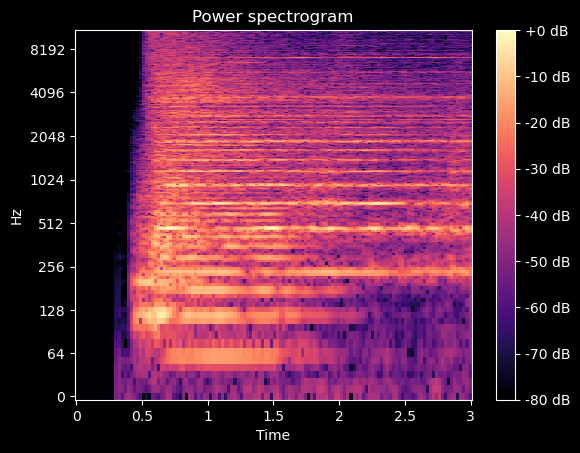
Power Spectral Density (PSD) is a measure of the power of a signal at different frequencies. The PSD is calculated using the Fourier Transform . The PSD is a useful representation of audio data because it is often easier to distinguish different sounds in the frequency domain than in the time domain.
import numpy as np = plt.subplots()= librosa.display.specshow(librosa.amplitude_to_db(np.abs (S), ref= np.max ),= 'log' , x_axis= 'time' , ax= ax); 'Power spectrogram' ); = ax, format = "%+2.0f dB" );
MFCCs
Mel-Frequency Cepstral Coefficients (MFCCs) are a representation of the short-term power spectrum of a sound. MFCCs are widely used in speech and audio processing because they capture the perceptually relevant features of the sound.
To put it simply, MFCCs are a way to represent audio data that mimics how humans perceive sound.
Using MFCCs, you can extract features from audio data that are more relevant for tasks like speech recognition or music classification.
The code below demonstrates how to load an audio file and compute its MFCCs.
import librosa= librosa.load('StarWars3.wav' )= librosa.feature.mfcc(y= y, sr= sr, n_mfcc= 13 )= mfcc.mean(axis= 1 ) # 13-dimensional vector
Note that this way, we can map each audio file to a fixed-size feature vector, which can then be used as input to machine learning models.

