Matrices

We denote matrices by bold capital letters (e.g., $X$, $Y$, and $Z$), and represent them in code by pd.DataFrame. The expression $\mathbf{A}\in {\mathbb{R}}^{m\times n}$ indicates that a matrix $\mathbf{\text{A}}$ contains $m\times n$ real-valued scalars, arranged as $m$ rows and $n$ columns. When $m=n$, we say that a matrix is square. Visually, we can illustrate any matrix as a table. To refer to an individual element, we subscript both the row and column indices, e.g., $a_{ij}$ is the value that belongs to $\mathbf{A}$’s $i^{th}$ row and $j^{th}$ column:

$$\begin{array}{r}\mathbf{A}=\left[\begin{array}{cccc}{a}_{11}& a_{12}& \cdots & a_{1n}\\ a_{21}& a_{22}& \cdots & a_{2n}\\ ⋮& ⋮& \ddots & ⋮\\ a_{m1}& a_{m2}& \cdots & a_{mn}\end{array}\right].\end{array}$$

import pandas as pd 

df = pd.DataFrame({'a': [1, 20, 3, 40], 'b': [50, 6, 70, 8]})

df.index = ['v1', 'v2', 'v3', 'v4']

df

	a	b
v1	1	50
v2	20	6
v3	3	70
v4	40	8

Geometry of Matrices

An (n, d) matrix can be interpreted as a collection of n vectors in d-dimensional space.

import seaborn as sns
from matplotlib import pyplot as plt

plt.style.use('dark_background')

ax = sns.scatterplot(x='a', y='b', data=df, s=100);
ax.set(title='Scatterplot of a vs b', xlabel='a', ylabel='b');

def annotate(row):
    plt.text(x=row['a']+0.05, y=row['b'], s=row.name, size=20);

df.apply(annotate, axis=1);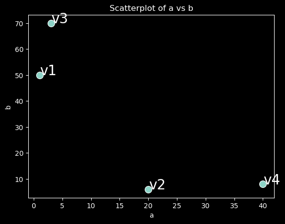

Transpose

Sometimes we want to flip the axes. When we exchange a matrix’s rows and columns, the result is called its transpose. Formally, we signify a matrix’s $\mathbf{\text{A}}$ transpose by ${\mathbf{A}}^{\mathrm{\top }}$ and if $\mathbf{B}={\mathbf{A}}^{\mathrm{\top }}$, then $b_{ij}=a_{ij}$ for all $i$ and $j$. Thus, the transpose of an $m\times n$ matrix is an $n\times m$ matrix:

$$\begin{array}{r}{\mathbf{A}}^{\mathrm{\top }}=\left[\begin{array}{cccc}{a}_{11}& a_{21}& \dots & a_{m1}\\ a_{12}& a_{22}& \dots & a_{m2}\\ ⋮& ⋮& \ddots & ⋮\\ a_{1n}& a_{2n}& \dots & a_{mn}\end{array}\right].\end{array}$$

In pandas, you can transpose a DataFrame with the .T attribute:

df.T

	v1	v2	v3	v4
a	1	20	3	40
b	50	6	70	8

Note that columns of original dataframe df are the same as index of df.T

df.columns == df.T.index

array([ True,  True])

df.T

	v1	v2	v3	v4
a	1	20	3	40
b	50	6	70	8

Matrix-Vector Products

Now that we know how to calculate dot products, we can begin to understand the product between an $m\times n$ matrix and an $n$-dimensional vector $\mathbf{x}$.

To start off, we visualize our matrix in terms of its row vectors

$$\begin{array}{r}\mathbf{A}=\left[\begin{array}{c}{\mathbf{a}}_1^{\mathrm{\top }}\\ {\mathbf{a}}_2^{\mathrm{\top }}\\ ⋮\\ {\mathbf{a}}_m^{\mathrm{\top }}\end{array}\right],\end{array}$$

where each ${\mathbf{a}}_i^{\mathrm{\top }}\in {\mathbb{R}}^n$ is a row vector representing the $i^{\text{th}}$ row of the matrix $\mathbf{A}$.

The matrix–vector product $\mathbf{A}\mathbf{x}$ is simply a column vector of length $m$ , whose $i^{th}$ element is the dot product ${\mathbf{a}}_i^{\mathrm{\top }}\mathbf{x}$

$$\begin{array}{r}\mathbf{A}\mathbf{x}=\left[\begin{array}{c}{\mathbf{a}}_1^{\mathrm{\top }}\\ {\mathbf{a}}_2^{\mathrm{\top }}\\ ⋮\\ {\mathbf{a}}_m^{\mathrm{\top }}\end{array}\right]\mathbf{x}=\left[\begin{array}{c}{\mathbf{a}}_1^{\mathrm{\top }}\mathbf{x}\\ {\mathbf{a}}_2^{\mathrm{\top }}\mathbf{x}\\ ⋮\\ {\mathbf{a}}_m^{\mathrm{\top }}\mathbf{x}\end{array}\right].\end{array}$$

We can think of multiplication with a matrix $\mathbf{A}\in {\mathbb{R}}^{m\times n}$ as a transformation that projects vectors from ${\mathbb{R}}^n$ to ${\mathbb{R}}^m$.

These transformations are remarkably useful. For example, we can represent rotations as multiplications by certain square matrices. Matrix–vector products also describe the key calculation involved in computing the outputs of each layer in a neural network given the outputs from the previous layer.

Finding similar vectors

Note that, given a vector $\mathbf{v}$, vector-matrix products can also be used to compute the similarity of $\mathbf{v}$ and each row ${\mathbf{a}}_i^{\mathrm{\top }}$ of matrix $\mathbf{A}$. This is because the matrix-vector product $\mathbf{A}\mathbf{v}$ will contain the dot products of $\mathbf{v}$ and each row in $\mathbf{A}$.

There is one thing to be careful about: recall that the formula for cosine similarity is:

$$\text{cos}(\theta )=\frac{\mathbf{a}\cdot \mathbf{b}}{\parallel \mathbf{a}\parallel \parallel \mathbf{b}\parallel }$$

The dot product (numerator, on the right hand side) is equal to the cosine of the angle between the two vectors when the vectors are normalized (i.e. each divided by their norms).

The example below shows how to compute the cosine similarity between a vector $\mathbf{v}$ and each row of matrix $\mathbf{A}$.

import pandas as pd
data = pd.read_csv('https://raw.githubusercontent.com/fahadsultan/csc272/main/data/chat_dataset.csv')

# creating bow representation
vocab = (' '.join(data['message'].values)).lower().split()
bow = pd.DataFrame(columns=vocab)
for word in vocab: 
    bow[word] = data['message'].apply(lambda msg: msg.count(word))

# l2 norm of a vector
def l2_norm(vec):
    return (sum(vec**2))**(1/2)

# bow where each row is a unit vectors i.e. ||row|| = 1
bow_unit = bow.apply(lambda row: row/l2_norm(row), axis=1)

# random message : I don't have an opinion on this
msg = bow_unit.iloc[20] 

# cosine similarity of first message with all other messages
msg_sim = bow_unit.dot(msg.T)
msg_sim.index = data['message']

msg_sim.sort_values(ascending=False)

message
I don't have an opinion on this           1.000000
I don't really have an opinion on this    0.984003
I have no strong opinion about this       0.971575
I have no strong opinions about this      0.971226
I have no strong opinion on this          0.969768
                                            ...   
I'm not sure what to do 😕                 0.204587
I'm not sure what to do next 🤷‍♂️         0.201635
I'm not sure what to do next 🤔            0.200593
The food was not good                     0.200295
The food was not very good                0.197220
Length: 584, dtype: float64

Matrix-Matrix Multiplication

Once you have gotten the hang of dot products and matrix–vector products, then matrix–matrix multiplication should be straightforward.

Say that we have two matrices $\mathbf{A}\in {\mathbb{R}}^{n\times k}$ and $\mathbf{B}\in {\mathbb{R}}^{k\times m}$:

$$\begin{array}{r}\mathbf{A}=\left[\begin{array}{cccc}{a}_{11}& a_{12}& \cdots & a_{1k}\\ a_{21}& a_{22}& \cdots & a_{2k}\\ ⋮& ⋮& \ddots & ⋮\\ a_{n1}& a_{n2}& \cdots & a_{nk}\end{array}\right],\mathbf{B}=\left[\begin{array}{cccc}{b}_{11}& b_{12}& \cdots & b_{1m}\\ b_{21}& b_{22}& \cdots & b_{2m}\\ ⋮& ⋮& \ddots & ⋮\\ b_{k1}& b_{k2}& \cdots & b_{km}\end{array}\right].\end{array}$$

Let ${\mathbf{a}}_i^{\mathrm{\top }}\in {\mathbb{R}}^k$ denote the row vector representing the $i^{\text{th}}$ row of the matrix $\mathbf{A}$ and let ${\mathbf{b}}_j\in {\mathbb{R}}^k$ denote the column vector from the $j^{\text{th}}$ column of the matrix $\mathbf{B}$ :

$$\begin{array}{r}\mathbf{A}=\left[\begin{array}{c}{\mathbf{a}}_1^{\mathrm{\top }}\\ {\mathbf{a}}_2^{\mathrm{\top }}\\ ⋮\\ {\mathbf{a}}_n^{\mathrm{\top }}\end{array}\right],\mathbf{B}=\left[\begin{array}{cccc}{\mathbf{b}}_1& {\mathbf{b}}_2& \cdots & {\mathbf{b}}_m\end{array}\right].\end{array}$$

To form the matrix product $\mathbf{C}\in {\mathbb{R}}^{n\times m}$ , we simply compute each element $c_{ij}$ as the dot product between the $i^{\text{th}}$ row of $\mathbf{A}$ and the $i^{\text{th}}$ column of $\mathbf{B}$ , i.e., ${\mathbf{a}}_i^{\mathrm{\top }}{\mathbf{b}}_j$ :

$$\begin{array}{r}\mathbf{C}=\mathbf{AB}=\left[\begin{array}{c}{\mathbf{a}}_1^{\mathrm{\top }}\\ {\mathbf{a}}_2^{\mathrm{\top }}\\ ⋮\\ {\mathbf{a}}_n^{\mathrm{\top }}\end{array}\right]\left[\begin{array}{cccc}{\mathbf{b}}_1& {\mathbf{b}}_2& \cdots & {\mathbf{b}}_m\end{array}\right]=\left[\begin{array}{cccc}{\mathbf{a}}_1^{\mathrm{\top }}{\mathbf{b}}_1& {\mathbf{a}}_1^{\mathrm{\top }}{\mathbf{b}}_2& \cdots & {\mathbf{a}}_1^{\mathrm{\top }}{\mathbf{b}}_m\\ {\mathbf{a}}_2^{\mathrm{\top }}{\mathbf{b}}_1& {\mathbf{a}}_2^{\mathrm{\top }}{\mathbf{b}}_2& \cdots & {\mathbf{a}}_2^{\mathrm{\top }}{\mathbf{b}}_m\\ ⋮& ⋮& \ddots & ⋮\\ {\mathbf{a}}_n^{\mathrm{\top }}{\mathbf{b}}_1& {\mathbf{a}}_n^{\mathrm{\top }}{\mathbf{b}}_2& \cdots & {\mathbf{a}}_n^{\mathrm{\top }}{\mathbf{b}}_m\end{array}\right].\end{array}$$

We can think of the matrix–matrix multiplication $\mathbf{AB}$ as performing $m$ matrix–vector products or $m\times n$ dot products and stitching the results together to form an $m\times n$ matrix. In the following snippet, we perform matrix multiplication on A and B. Here, A is a matrix with two rows and three columns, and B is a matrix with three rows and four columns. After multiplication, we obtain a matrix with two rows and four columns.

Computing similarity / distance matrix

Note that, given two matrices $\mathbf{A}$ and $\mathbf{B}$, matrix-matrix products can also be used to compute the similarity between each row ${\mathbf{a}}_i^{\mathrm{\top }}$ of matrix $\mathbf{A}$ and each row ${\mathbf{b}}_j^{\mathrm{\top }}$ of matrix $\mathbf{B}$. This is because the matrix-matrix product $\mathbf{A}\mathbf{B}$ will contain the dot products of each pair of rows in $\mathbf{A}$ and $\mathbf{B}$.

similarity_matrix = bow_unit.dot(bow_unit.T)

similarity_matrix.shape

(584, 584)

similarity_matrix.head()

	0	1	2	3	4	5	6	7	8	9	...	574	575	576	577	578	579	580	581	582	583
0	1.000000	0.568191	0.453216	0.565809	0.612787	0.608156	0.377769	0.631309	0.793969	0.642410	...	0.516106	0.612624	0.660911	0.490580	0.845518	0.573549	0.648564	0.629598	0.594468	0.570452
1	0.568191	1.000000	0.508206	0.928580	0.687137	0.681944	0.423604	0.707906	0.551139	0.720354	...	0.573755	0.686954	0.741100	0.546166	0.801864	0.643139	0.721001	0.705988	0.652357	0.639666
2	0.453216	0.508206	1.000000	0.506075	0.548093	0.707857	0.778316	0.621438	0.538883	0.648861	...	0.457088	0.547948	0.650512	0.443105	0.593732	0.512998	0.574392	0.605515	0.520351	0.609064
3	0.565809	0.928580	0.506075	1.000000	0.685614	0.679085	0.421828	0.704938	0.548828	0.717334	...	0.571349	0.684074	0.737993	0.543876	0.798502	0.640442	0.717978	0.703027	0.649622	0.638039
4	0.612787	0.687137	0.548093	0.685614	1.000000	0.735468	0.273748	0.559585	0.714100	0.599091	...	0.926494	0.825530	0.806139	0.933257	0.802775	0.945544	0.931874	0.913601	0.928473	0.690556

5 rows × 584 columns

from matplotlib import pyplot as plt
plt.imshow(similarity_matrix, cmap='Greens')
plt.colorbar();
plt.title("Similarity Matrix: Each cell contains cosine \nsimilarity between two messages");
plt.xlabel("Message Index");
plt.ylabel("Message Index");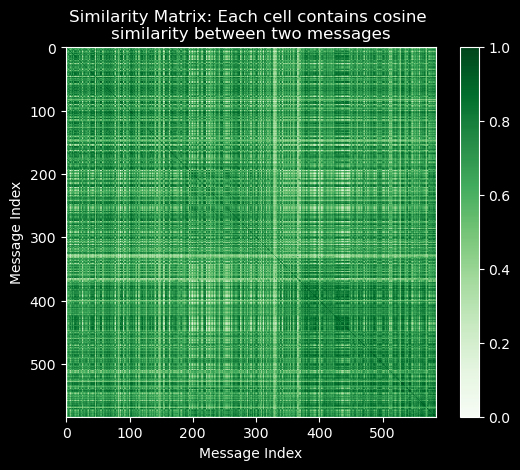

Note how 1. the similarity matrix is symmetric, i.e. $si{m}_{ij}=si{m}_{ji}$ and 2. the diagonal elements are all 1, i.e. $si{m}_{ii}=1$.

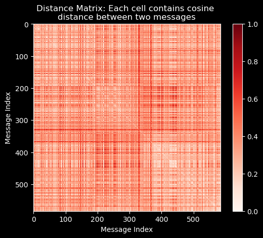
distance_matrix = 1 - bow_unit.dot(bow_unit.T)

from matplotlib import pyplot as plt
plt.imshow(distance_matrix, cmap='Reds')
plt.colorbar();
plt.title("Distance Matrix: Each cell contains cosine \ndistance between two messages");
plt.xlabel("Message Index");
plt.ylabel("Message Index");