Transformers for images

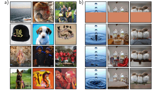
ImageGPT. a) Images generated from the autoregressive ImageGPT model. The top-left pixel is drawn from the estimated empirical distribution at this position. Subsequent pixels are generated in turn, conditioned on the previous ones, working along the rows until the bottom-right of the image is reached. For each pixel, the transformer decoder generates a conditional distribution as in equation 12.15, and a sample is drawn. The extended sequence is then fed back into the network to generate the next pixel, and so on. b) Image completion. In each case, the lower half of the image is removed (top row), and ImageGPT completes the remaining part pixel by pixel (three different completions shown). Adapted from https://openai.com/blog/image-gpt/.

ImageGPT

Vision Transformer (ViT)

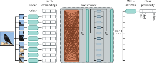
Vision transformer. The Vision Transformer (ViT) breaks the image into a grid of patches (16×16 in the original implementation). Each of these is projected via a learned linear transformation to become a patch embedding. These patch embeddings are fed into a transformer encoder network, and the token is used to predict the class probabilities.

Multi-scale vision transformers

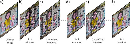
Shifted window (SWin) transformer (Liu et al., 2021c). a) Original image. b) The SWin transformer breaks the image into a grid of windows and each of these windows into a sub-grid of patches. The transformer network applies self-attention to the patches within each window independently (i.e., patches only attend to other patches in the same window). c) Each alternate layer shifts the windows so that the subsets of patches that interact with one another change, and information can propagate across the whole image. d) After several layers, the 2×2 blocks of patch representations are concatenated to increase the effective patch (and window) size. e) Alternate layers use shifted windows at this new lower resolution. f) Eventually, the resolution is such that there is just a single window, and the patches span the entire image.

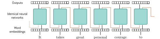
Recurrent neural networks (RNNs). The word embeddings are passed sequentially through a series of identical neural networks. Each network has two outputs; one is the output embedding, and the other (orange arrows) feeds back into the next neural network, along with the next word embedding. Each output embedding contains information about the word itself and its context in the preceding sentence fragment. In principle, the final output contains information about the entire sentence and could be used to support classification tasks similarly to the token in a transformer encoder model. However, RNNs sometimes gradually “forget” about tokens that are further back in time.

Equations

\[\begin{eqnarray}\label{eq:transformer_position_quad} \mbox{{\bf Sa}}[\mathbf{X}] =\mathbf{V}\cdot\mbox{\bf Softmax}\left[\frac{\mathbf{K}^{T}\mathbf{Q}}{\sqrt{D}_{q}}\right], \end{eqnarray}\]

\[\begin{eqnarray} \mathbf{V} &=& \boldsymbol\beta_{v}\mathbf{1}^{T}+\boldsymbol\Omega_{\textit{v}}\mathbf{X}\nonumber \\ \mathbf{Q} &=& \boldsymbol\beta_{q}\mathbf{1}^{T}+\boldsymbol\Omega_{\textit{q}}(\mathbf{X}+\boldsymbol\Pi)\nonumber \\ \mathbf{K} &=& \boldsymbol\beta_{k}\mathbf{1}^{T}+\boldsymbol\Omega_{\textit{k}}(\mathbf{X}+\boldsymbol\Pi). \end{eqnarray}\]

\[\begin{eqnarray} \mbox{\bf Sa}[\mathbf{X}\mathbf{P}] = \mbox{\bf Sa}[\mathbf{X}]\mathbf{P}. \end{eqnarray}\]

\[\begin{eqnarray} y_{i} = \mbox{softmax}_{i}[\mathbf{z}] = \frac{\exp[z_{i}]}{\sum_{j=1}^{5}\exp[z_{j}]}, \end{eqnarray}\]

\[\begin{eqnarray} a[\mathbf{x}_{m},\mathbf{x}_{n}] = \mbox{softmax}_{m}\left[\mathbf{k}_{\bullet}^T\mathbf{q}_{n}\right] = \frac{\exp\left[\mathbf{k}_m^T\mathbf{q}_{n}\right]}{\sum_{m'=1}^{N}\exp\left[\mathbf{k}_{m'}^{T}\mathbf{q}_{n} \right]}. \end{eqnarray}\]