# Run this if you're in a Colab to install MNIST 1D repository
!pip install git+https://github.com/greydanus/mnist1d
Find wider minima
Applying noise
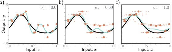
Dropout can be interpreted as applying multiplicative Bernoulli noise to the network activations. This leads to the idea of applying noise to other parts of the network during training to make the final model more robust. One option is to add noise to the input data; this smooths out the learned function (figure 9.10). For regression problems, it can be shown to be equivalent to adding a regularizing term that penalizes the derivatives of the network’s output with respect to its input. An extreme variant is adversarial training, in which the optimization algorithm actively searches for small perturbations of the input that cause large changes to the output. These can be thought of as worst-case additive noise vectors. A second possibility is to add noise to the weights. This encourages the network to make sensible predictions even for small perturbations of the weights. The result is that the training converges to local minima in the middle of wide, flat regions, where changing the individual weights does not matter much. Finally, we can perturb the labels. The maximum-likelihood criterion for multiclass classification aims to predict the correct class with absolute certainty (equation 5.24). To this end, the final network activations (i.e., before the softmax function) are pushed to very large values for the correct class and very small values for the wrong classes. We could discourage this overconfident behavior by assuming that a proportion ρ of the training labels are incorrect and belong with equal probability to the other classes. This could be done by randomly changing the labels at each training iteration. However, the same end can be achieved by changing the loss function to minimize the cross- entropy between the predicted distribution and a distribution where the true label has probability 1−ρ, and the other classes have equal probability. This is known as label smoothing and improves generalization in diverse scenarios.
Augmentation
Transfer learning improves performance by exploiting a different dataset. Multi-task learning improves performance using additional labels. A third option is to expand the dataset. We can often transform each input data example in such a way that the label stays the same. For example, we might aim to determine if there is a bird in an image (figure 9.13). Here, we could rotate, flip, blur, or manipulate the color balance of the image, and the label “bird” remains valid. Similarly, for tasks where the input is text, we can substitute synonyms or translate to another language and back again. For tasks where the input is audio, we can amplify or attenuate different frequency bands.
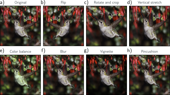
Data augmentation. For some problems, each data example can be transformed to augment the dataset. a) Original image. b–h) Various geometric and photometric transformations of this image. For image classification, all these images still have the same label, “bird.” Adapted from Wu et al. (2015a).
Generating extra training data in this way is known as data augmentation. The aim is to teach the model to be indifferent to these irrelevant data transformations.
import torch, torch.nn as nn
from torch.utils.data import TensorDataset, DataLoader
from torch.optim.lr_scheduler import StepLR
import numpy as np
import matplotlib.pyplot as plt
import mnist1d
import random
args = mnist1d.data.get_dataset_args()
data = mnist1d.data.get_dataset(args, path='./mnist1d_data.pkl', download=False, regenerate=False)
# The training and test input and outputs are in
# data['x'], data['y'], data['x_test'], and data['y_test']
print("Examples in training set: {}".format(len(data['y'])))
print("Examples in test set: {}".format(len(data['y_test'])))
print("Length of each example: {}".format(data['x'].shape[-1]))D_i = 40 # Input dimensions
D_k = 200 # Hidden dimensions
D_o = 10 # Output dimensions
# Define a model with two hidden layers of size 200
# And ReLU activations between them
model = nn.Sequential(
nn.Linear(D_i, D_k),
nn.ReLU(),
nn.Linear(D_k, D_k),
nn.ReLU(),
nn.Linear(D_k, D_o))
def weights_init(layer_in):
# Initialize the parameters with He initialization
if isinstance(layer_in, nn.Linear):
nn.init.kaiming_uniform_(layer_in.weight)
layer_in.bias.data.fill_(0.0)# choose cross entropy loss function (equation 5.24)
loss_function = torch.nn.CrossEntropyLoss()
# construct SGD optimizer and initialize learning rate and momentum
optimizer = torch.optim.SGD(model.parameters(), lr = 0.05, momentum=0.9)
# object that decreases learning rate by half every 10 epochs
scheduler = StepLR(optimizer, step_size=10, gamma=0.5)
# create 100 dummy data points and store in data loader class
x_train = torch.tensor(data['x'].astype('float32'))
y_train = torch.tensor(data['y'].transpose().astype('long'))
x_test= torch.tensor(data['x_test'].astype('float32'))
y_test = torch.tensor(data['y_test'].astype('long'))
# load the data into a class that creates the batches
data_loader = DataLoader(TensorDataset(x_train,y_train), batch_size=100, shuffle=True, worker_init_fn=np.random.seed(1))
# Initialize model weights
model.apply(weights_init)
# loop over the dataset n_epoch times
n_epoch = 50
# store the loss and the % correct at each epoch
errors_train = np.zeros((n_epoch))
errors_test = np.zeros((n_epoch))
for epoch in range(n_epoch):
# loop over batches
for i, batch in enumerate(data_loader):
# retrieve inputs and labels for this batch
x_batch, y_batch = batch
# zero the parameter gradients
optimizer.zero_grad()
# forward pass -- calculate model output
pred = model(x_batch)
# compute the loss
loss = loss_function(pred, y_batch)
# backward pass
loss.backward()
# SGD update
optimizer.step()
# Run whole dataset to get statistics -- normally wouldn't do this
pred_train = model(x_train)
pred_test = model(x_test)
_, predicted_train_class = torch.max(pred_train.data, 1)
_, predicted_test_class = torch.max(pred_test.data, 1)
errors_train[epoch] = 100 - 100 * (predicted_train_class == y_train).float().sum() / len(y_train)
errors_test[epoch]= 100 - 100 * (predicted_test_class == y_test).float().sum() / len(y_test)
print(f'Epoch {epoch:5d}, train error {errors_train[epoch]:3.2f}, test error {errors_test[epoch]:3.2f}')# Plot the results
fig, ax = plt.subplots()
ax.plot(errors_train,'r-',label='train')
ax.plot(errors_test,'b-',label='test')
ax.set_ylim(0,100); ax.set_xlim(0,n_epoch)
ax.set_xlabel('Epoch'); ax.set_ylabel('Error')
ax.set_title('Train Error %3.2f, Test Error %3.2f'%(errors_train[-1],errors_test[-1]))
ax.legend()
plt.show()The best test performance is about 33%. Let’s see if we can improve on that by augmenting the data.
def augment(input_vector):
  # Create output vector
  data_out = np.zeros_like(input_vector)

  # TODO:  Shift the input data by a random offset
  # (rotating, so points that would go off the end, are added back to the beginning)
  # Replace this line:
  data_out = np.zeros_like(input_vector) ;

  # TODO:    # Randomly scale the data by a factor drawn from a uniform distribution over [0.8,1.2]
  # Replace this line:
  data_out = np.array(data_out)

  return data_out
n_data_orig = data['x'].shape[0]
# We'll double the amount of data
n_data_augment = n_data_orig+4000
augmented_x = np.zeros((n_data_augment, D_i))
augmented_y = np.zeros(n_data_augment)
# First n_data_orig rows are original data
augmented_x[0:n_data_orig,:] = data['x']
augmented_y[0:n_data_orig] = data['y']
# Fill in rest of with augmented data
for c_augment in range(n_data_orig, n_data_augment):
# Choose a data point randomly
random_data_index = random.randint(0, n_data_orig-1)
# Augment the point and store
augmented_x[c_augment,:] = augment(data['x'][random_data_index,:])
augmented_y[c_augment] = data['y'][random_data_index]# choose cross entropy loss function (equation 5.24)
loss_function = torch.nn.CrossEntropyLoss()
# construct SGD optimizer and initialize learning rate and momentum
optimizer = torch.optim.SGD(model.parameters(), lr = 0.05, momentum=0.9)
# object that decreases learning rate by half every 50 epochs
scheduler = StepLR(optimizer, step_size=10, gamma=0.5)
# create 100 dummy data points and store in data loader class
x_train = torch.tensor(augmented_x.astype('float32'))
y_train = torch.tensor(augmented_y.transpose().astype('long'))
x_test= torch.tensor(data['x_test'].astype('float32'))
y_test = torch.tensor(data['y_test'].astype('long'))
# load the data into a class that creates the batches
data_loader = DataLoader(TensorDataset(x_train,y_train), batch_size=100, shuffle=True, worker_init_fn=np.random.seed(1))
# Initialize model weights
model.apply(weights_init)
# loop over the dataset n_epoch times
n_epoch = 50
# store the loss and the % correct at each epoch
errors_train_aug = np.zeros((n_epoch))
errors_test_aug = np.zeros((n_epoch))
for epoch in range(n_epoch):
# loop over batches
for i, batch in enumerate(data_loader):
# retrieve inputs and labels for this batch
x_batch, y_batch = batch
# zero the parameter gradients
optimizer.zero_grad()
# forward pass -- calculate model output
pred = model(x_batch)
# compute the loss
loss = loss_function(pred, y_batch)
# backward pass
loss.backward()
# SGD update
optimizer.step()
# Run whole dataset to get statistics -- normally wouldn't do this
pred_train = model(x_train)
pred_test = model(x_test)
_, predicted_train_class = torch.max(pred_train.data, 1)
_, predicted_test_class = torch.max(pred_test.data, 1)
errors_train_aug[epoch] = 100 - 100 * (predicted_train_class == y_train).float().sum() / len(y_train)
errors_test_aug[epoch]= 100 - 100 * (predicted_test_class == y_test).float().sum() / len(y_test)
print(f'Epoch {epoch:5d}, train error {errors_train_aug[epoch]:3.2f}, test error {errors_test_aug[epoch]:3.2f}')# Plot the results
fig, ax = plt.subplots()
ax.plot(errors_train,'r-',label='train')
ax.plot(errors_test,'b-',label='test')
ax.plot(errors_test_aug,'g-',label='test (augmented)')
ax.set_ylim(0,100); ax.set_xlim(0,n_epoch)
ax.set_xlabel('Epoch'); ax.set_ylabel('Error')
ax.set_title('TrainError %3.2f, Test Error %3.2f'%(errors_train_aug[-1],errors_test_aug[-1]))
ax.legend()
plt.show()Hopefully, you should see an improvement in performance when we augment the data.