where \(\mathbf{m}_t\) is the momentum (which drives the update at iteration t), \(\beta \in[0,1)\) controls the degree to which the gradient is smoothed over time, and \(\alpha\) is the learning rate.
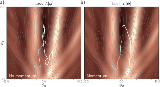
The recursive formulation of the momentum calculation means that the gradient step is an infinite weighted sum of all the previous gradients, where the weights get smaller as we move back in time.
The effective learning rate increases if all thefse gradients are aligned over multiple iterations but decreases if the gradient direction repeatedly changes as the terms in the sum cancel out. The overall effect is a smoother trajectory and reduced oscillatory behavior in valleys.
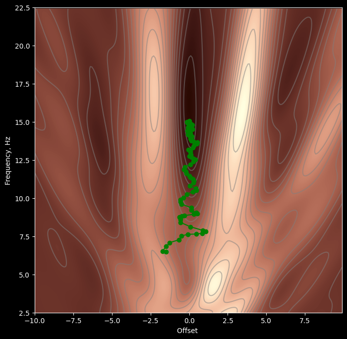
Figure 6.7 Stochastic gradient descent with momentum. a) Regular stochastic descent takes a very indirect path toward the minimum. b) With a momentum term, the change at the current step is a weighted combination of the previous change and the gradient computed from the batch. This smooths out the trajectory and increases the speed of convergence.
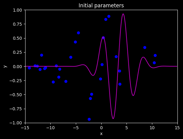
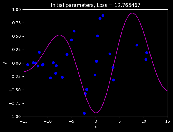
# import librariesimport numpy as npimport matplotlib.pyplot as pltfrom matplotlib import cmfrom matplotlib.colors import ListedColormapplt.style.use('dark_background')# Let's create our training data of 30 pairs {x_i, y_i}# We'll try to fit the Gabor model to these datadata = np.array([[-1.920e+00,-1.422e+01,1.490e+00,-1.940e+00,-2.389e+00,-5.090e+00,-8.861e+00,3.578e+00,-6.010e+00,-6.995e+00,3.634e+00,8.743e-01,-1.096e+01,4.073e-01,-9.467e+00,8.560e+00,1.062e+01,-1.729e-01,1.040e+01,-1.261e+01,1.574e-01,-1.304e+01,-2.156e+00,-1.210e+01,-1.119e+01,2.902e+00,-8.220e+00,-1.179e+01,-8.391e+00,-4.505e+00], [-1.051e+00,-2.482e-02,8.896e-01,-4.943e-01,-9.371e-01,4.306e-01,9.577e-03,-7.944e-02 ,1.624e-01,-2.682e-01,-3.129e-01,8.303e-01,-2.365e-02,5.098e-01,-2.777e-01,3.367e-01,1.927e-01,-2.222e-01,6.352e-02,6.888e-03,3.224e-02,1.091e-02,-5.706e-01,-5.258e-02,-3.666e-02,1.709e-01,-4.805e-02,2.008e-01,-1.904e-01,5.952e-01]])# Let's define our modeldef model(phi,x): sin_component = np.sin(phi[0] +0.06* phi[1] * x) gauss_component = np.exp(-(phi[0] +0.06* phi[1] * x) * (phi[0] +0.06* phi[1] * x) /32) y_pred= sin_component * gauss_componentreturn y_pred# Draw modeldef draw_model(data,model,phi,title=None): x_model = np.arange(-15,15,0.1) y_model = model(phi,x_model) fix, ax = plt.subplots() ax.plot(data[0,:],data[1,:],'bo') ax.plot(x_model,y_model,'m-') ax.set_xlim([-15,15]);ax.set_ylim([-1,1]) ax.set_xlabel('x'); ax.set_ylabel('y')if title isnotNone: ax.set_title(title) plt.show()# Initialize the parameters and draw the modelphi = np.zeros((2,1))phi[0] =-5# Horizontal offsetphi[1] =25# Frequencydraw_model(data,model,phi, "Initial parameters")
As before, we compute the gradient vector for a given set of parameters:
# These came from writing out the expression for the sum of squares loss and taking the# derivative with respect to phi0 and phi1. It was a lot of hassle to get it right!def gabor_deriv_phi0(data_x,data_y,phi0, phi1): x =0.06* phi1 * data_x + phi0 y = data_y cos_component = np.cos(x) sin_component = np.sin(x) gauss_component = np.exp(-0.5* x *x /16) deriv = cos_component * gauss_component - sin_component * gauss_component * x /16 deriv =2* deriv * (sin_component * gauss_component - y)return np.sum(deriv)def gabor_deriv_phi1(data_x, data_y,phi0, phi1): x =0.06* phi1 * data_x + phi0 y = data_y cos_component = np.cos(x) sin_component = np.sin(x) gauss_component = np.exp(-0.5* x *x /16) deriv =0.06* data_x * cos_component * gauss_component -0.06* data_x*sin_component * gauss_component * x /16 deriv =2*deriv * (sin_component * gauss_component - y)return np.sum(deriv)def compute_gradient(data_x, data_y, phi): dl_dphi0 = gabor_deriv_phi0(data_x, data_y, phi[0],phi[1]) dl_dphi1 = gabor_deriv_phi1(data_x, data_y, phi[0],phi[1])# Return the gradientreturn np.array([[dl_dphi0],[dl_dphi1]])
Let’s first run standard stochastic gradient descent.
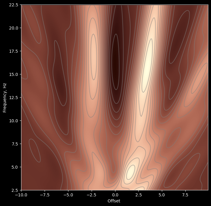
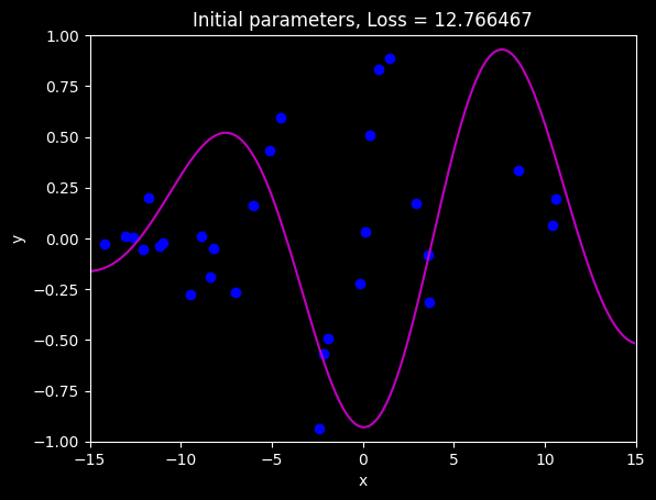
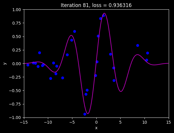
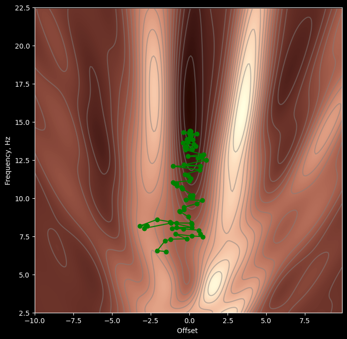
# Set the random number generator so you always get same numbers (disable if you don't want this)np.random.seed(1)# Initialize the parametersn_steps =81batch_size =5alpha =0.6phi_all = np.zeros((2,n_steps+1))phi_all[0,0] =-1.5phi_all[1,0] =6.5# Measure loss and draw initial modelloss = compute_loss(data[0,:], data[1,:], model, phi_all[:,0:1])draw_model(data,model,phi_all[:,0:1], "Initial parameters, Loss = %f"%(loss))for c_step inrange (n_steps):# Choose random batch indices batch_index = np.random.permutation(data.shape[1])[0:batch_size]# Compute the gradient gradient = compute_gradient(data[0,batch_index], data[1,batch_index], phi_all[:,c_step:c_step+1] )# Update the parameters phi_all[:,c_step+1:c_step+2] = phi_all[:,c_step:c_step+1] - alpha * gradientloss = compute_loss(data[0,:], data[1,:], model, phi_all[:,c_step+1:c_step+2])draw_model(data,model,phi_all[:,c_step+1], "Iteration %d, loss = %f"%(c_step+1,loss))draw_loss_function(compute_loss, data, model,phi_all)
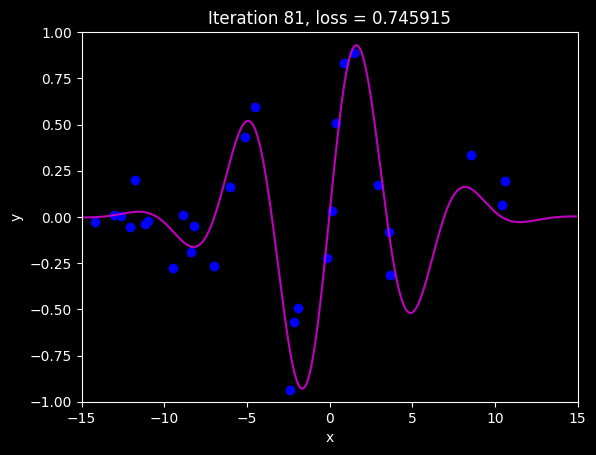
Now let’s add momentum (equation 6.11)
# Set the random number generator so you always get same numbers (disable if you don't want this)np.random.seed(1)# Initialize the parametersn_steps =81batch_size =5alpha =0.6beta =0.6momentum = np.zeros([2,1])phi_all = np.zeros((2,n_steps+1))phi_all[0,0] =-1.5phi_all[1,0] =6.5# Measure loss and draw initial modelloss = compute_loss(data[0,:], data[1,:], model, phi_all[:,0:1])draw_model(data,model,phi_all[:,0:1], "Initial parameters, Loss = %f"%(loss))for c_step inrange (n_steps):# Choose random batch indices batch_index = np.random.permutation(data.shape[1])[0:batch_size]# Compute the gradient gradient = compute_gradient(data[0,batch_index], data[1,batch_index], phi_all[:,c_step:c_step+1])# TODO -- calculate momentum - replace the line below momentum = beta * momentum + (1-beta) * gradient# Update the parameters phi_all[:,c_step+1:c_step+2] = phi_all[:,c_step:c_step+1] - alpha * momentumloss = compute_loss(data[0,:], data[1,:], model, phi_all[:,c_step+1:c_step+2])draw_model(data,model,phi_all[:,c_step+1], "Iteration %d, loss = %f"%(c_step+1,loss))draw_loss_function(compute_loss, data, model,phi_all)