# Imports math library
import numpy as np
# Imports plotting library
import matplotlib.pyplot as plt
# Import math Library
import math

plt.style.use('dark_background')

# Define the Rectified Linear Unit (ReLU) function
def ReLU(preactivation):
  activation = preactivation.clip(0.0)
  return activation

# Define a shallow neural network
def shallow_nn(x, beta_0, omega_0, beta_1, omega_1):
    # Make sure that input data is (1 x n_data) array
    n_data = x.size
    x = np.reshape(x,(1,n_data))

    # This runs the network for ALL of the inputs, x at once so we can draw graph
    h1 = ReLU(np.matmul(beta_0,np.ones((1,n_data))) + np.matmul(omega_0,x))
    model_out = np.matmul(beta_1,np.ones((1,n_data))) + np.matmul(omega_1,h1)
    return model_out


# Get parameters for model -- we can call this function to easily reset them
def get_parameters():
  # And we'll create a network that approximately fits it
  beta_0 = np.zeros((3,1));  # formerly theta_x0
  omega_0 = np.zeros((3,1)); # formerly theta_x1
  beta_1 = np.zeros((1,1));  # formerly phi_0
  omega_1 = np.zeros((1,3)); # formerly phi_x

  beta_0[0,0] = 0.3; beta_0[1,0] = -1.0; beta_0[2,0] = -0.5
  omega_0[0,0] = -1.0; omega_0[1,0] = 1.8; omega_0[2,0] = 0.65
  beta_1[0,0] = 2.6;
  omega_1[0,0] = -24.0; omega_1[0,1] = -8.0; omega_1[0,2] = 50.0

  return beta_0, omega_0, beta_1, omega_1


# Utility function for plotting data
def plot_binary_classification(x_model, out_model, lambda_model, x_data = None, y_data = None, title= None):
  # Make sure model data are 1D arrays
  x_model = np.squeeze(x_model)
  out_model = np.squeeze(out_model)
  lambda_model = np.squeeze(lambda_model)

  fig, ax = plt.subplots(1,2)
  fig.set_size_inches(7.0, 3.5)
  fig.tight_layout(pad=3.0)
  ax[0].plot(x_model,out_model)
  ax[0].set_xlabel(r'Input, $x$'); ax[0].set_ylabel(r'Model output')
  ax[0].set_xlim([0,1]);ax[0].set_ylim([-4,4])
  if title is not None:
    ax[0].set_title(title)
  ax[1].plot(x_model,lambda_model)
  ax[1].set_xlabel(r'Input, $x$'); ax[1].set_ylabel(r'$y$ or Pr(y=1|x)')
  ax[1].set_xlim([0,1]);ax[1].set_ylim([-0.05,1.05])
  if title is not None:
    ax[1].set_title(title)
  if x_data is not None:
    ax[1].plot(x_data, y_data, 'ko')
  plt.show()
Example 2: binary classification
In binary classification, the goal is to assign the data \(x\) to one of two discrete classes \(y \in {0,1}\). In this context, we refer to y as a label. Examples of binary classification include
predicting whether a restaurant review is positive (\(y = 1\)) or negative (\(y = 0\)) from text data \(x\) and
predicting whether a tumor is present (\(y = 1\)) or absent (\(y = 0\)) from an MRI scan \(x\).
Once again, we follow the recipe to construct the loss function. First, we choose a probability distribution over the output space \(y\in{0,1}\).
A suitable choice is the Bernoulli distribution, which is defined on the domain \({0,1}\).
This has a single parameter \(\lambda \in [0,1]\) that represents the probability that \(y\) takes the value 1 :
\[\begin{eqnarray} Pr(y|\lambda) = \begin{cases} 1-\lambda & \quad y =0 \\ \lambda & \quad y= 1\end{cases} \end{eqnarray}\]
which can equivalently be written as:
\[\begin{eqnarray} Pr(y|\lambda) = (1-\lambda)^{1-y}\cdot \lambda^{y}. \end{eqnarray}\]
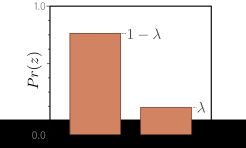
Bernoulli distribution.
The Bernoulli distribution is defined on the domain \(z \in \{0, 1\}\) and has a single parameter \(\lambda\) that denotes the probability of observing \(z = 1\).
It follows that the probability of observing \(z = 0\) is \(1 − \lambda\).
Second, we set the machine learning model \(f[x,\phi]\) to predict the single distribution parameter \(\lambda\).
However, \(\lambda\) can only take values in the range \([0,1]\), and we cannot guarantee that the network output will lie in this range.
Consequently, we pass the network output through a function that maps the real numbers \(\mathbb{R}\) to \([0,1]\).
A suitable function is the logistic sigmoid:
\[\begin{eqnarray}\label{eq:logistic_sigmoid} \mbox{sig}[z] = \frac{1}{1+\exp[-z]}. \end{eqnarray}\]
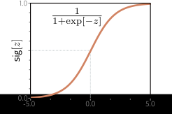
Logistic sigmoid function.
This function maps the real line \(z \in \mathbb{R}\) to numbers between zero and one, so \(\mbox{sig}[z] \in [0, 1]\).
An input of 0 is mapped to 0.5.
Negative inputs are mapped to numbers below 0.5, and positive inputs to numbers above 0.5.
Hence, we predict the distribution parameter as \(\lambda= \mbox{sig}[\mbox{f}[\mathbf{x},\boldsymbol\phi]]\).
The likelihood is now:
\[\begin{eqnarray}\label{eq:loss_binary} Pr(y|\mathbf{x}) = (1-\mbox{sig}[\mbox{f}[\mathbf{x},\boldsymbol\phi]])^{1-y}\cdot \mbox{sig}[\mbox{f}[\mathbf{x},\boldsymbol\phi]]^y. \end{eqnarray}\]
This is depicted in figure below for a shallow neural network model. The loss function is the negative log-likelihood of the training set:
\[\begin{eqnarray}\label{eq:loss_binary_cross_entropy} L[\boldsymbol\phi] = \sum_{i=1}^{I}-(1-y_{i})\log\Bigl[1-\mbox{sig}[\mbox{f}[\mathbf{x}_i,\boldsymbol\phi]]\Bigr] - y_{i}\log\Bigl[\mbox{sig}[\mbox{f}[\mathbf{x}_i,\boldsymbol\phi]]\Bigr]. \end{eqnarray}\]
This is known as the binary cross-entropy loss.
The transformed model output \(sig[f[x,\phi]]\) predicts the parameter \(\lambda\) of the Bernoulli distribution.
This represents the probability that \(y = 1\), and it follows that \(1−\lambda\) represents the probability that \(y= 0\). When we perform inference, we may want a point estimate of \(y\), so we set \(y= 1\) if \(\lambda>0.5\) and \(y= 0\) otherwise.
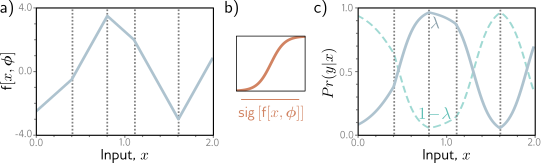
Binary classification model.
The network output is a piecewise linear function that can take arbitrary real values.
This is transformed by the logistic sigmoid function, which compresses these values to the range \([0, 1]\).
The transformed output predicts the probability \(\lambda\) that \(y = 1\) (solid line). The probability that \(y = 0\) is hence \(1 − \lambda\) (dashed line). For any fixed \(x\) (vertical slice), we retrieve the two values of a Bernoulli distribution. The loss function favors model parameters that produce large values of \(\lambda\) at positions \(x_i\) that are associated with positive examples \(y_i = 1\) and small values of \(\lambda\) at positions associated with negative examples \(y_i = 0\).
In binary classification tasks, the network predicts the probability of the output belonging to class 1. Since probabilities must lie in [0,1] and the network can output arbitrary values, we map the network through a sigmoid function that ensures the range is valid.
# Sigmoid function that maps [-infty,infty] to [0,1]
def sigmoid(model_out):

  sig_model_out = 1 / (1 + np.exp(-model_out))

  return sig_model_out


# Let's create some 1D training data
x_train = np.array([0.09291784,0.46809093,0.93089486,0.67612654,0.73441752,0.86847339,\
                   0.49873225,0.51083168,0.18343972,0.99380898,0.27840809,0.38028817,\
                   0.12055708,0.56715537,0.92005746,0.77072270,0.85278176,0.05315950,\
                   0.87168699,0.58858043])
y_train = np.array([0,1,1,0,0,1,\
                    1,0,0,1,0,1,\
                    0,1,1,0,1,0, \
                    1,1])

# Get parameters for the model
beta_0, omega_0, beta_1, omega_1 = get_parameters()

# Define a range of input values
x_model = np.arange(0,1,0.01)
# Run the model to get values to plot and plot it.
model_out= shallow_nn(x_model, beta_0, omega_0, beta_1, omega_1)
lambda_model = sigmoid(model_out)
plot_binary_classification(x_model, model_out, lambda_model, x_train, y_train)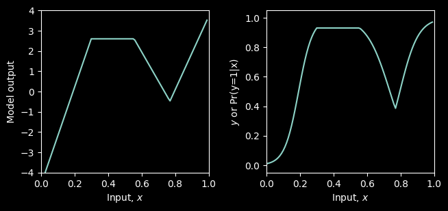
The left is model output and the right is the model output after the sigmoid has been applied, so it now lies in the range [0,1] and represents the probability, that y=1. The black dots show the training data. We’ll compute the likelihood and the negative log likelihood.
# Return probability under Bernoulli distribution for observed class y
def bernoulli_distribution(y, lambda_param):

    prob = np.power(1-lambda_param, 1-y) * np.power(lambda_param, y)

    return prob


# Let's double check we get the right answer before proceeding
print("Correct answer = %3.3f, Your answer = %3.3f"%(0.8,bernoulli_distribution(0,0.2)))
print("Correct answer = %3.3f, Your answer = %3.3f"%(0.2,bernoulli_distribution(1,0.2)))
Correct answer = 0.800, Your answer = 0.800
Correct answer = 0.200, Your answer = 0.200Now let’s compute the likelihood using this function
# Return the likelihood of all of the data under the model
def compute_likelihood(y_train, lambda_param):

  likelihood = np.prod(bernoulli_distribution(y_train, lambda_param))

  return likelihood
# Let's test this
beta_0, omega_0, beta_1, omega_1 = get_parameters()
# Use our neural network to predict the Bernoulli parameter lambda
model_out = shallow_nn(x_train, beta_0, omega_0, beta_1, omega_1)
lambda_train = sigmoid(model_out)
# Compute the likelihood
likelihood = compute_likelihood(y_train, lambda_train)
# Let's double check we get the right answer before proceeding
print("Correct answer = %9.9f, Your answer = %9.9f"%(0.000070237,likelihood))Correct answer = 0.000070237, Your answer = 0.000070237You can see that this gives a very small answer, even for this small 1D dataset, and with the model fitting quite well. This is because it is the product of several probabilities, which are all quite small themselves. This will get out of hand pretty quickly with real datasets – the likelihood will get so small that we can’t represent it with normal finite-precision math
This is why we use negative log likelihood
# Return the negative log likelihood of the data under the model
def compute_negative_log_likelihood(y_train, lambda_param):

  nll = -np.sum(y_train * np.log(lambda_param) + (1 - y_train) * np.log(1 - lambda_param))

  return nll


# Let's test this
beta_0, omega_0, beta_1, omega_1 = get_parameters()
# Use our neural network to predict the mean of the Gaussian
model_out = shallow_nn(x_train, beta_0, omega_0, beta_1, omega_1)
# Pass through the sigmoid function
lambda_train = sigmoid(model_out)
# Compute the log likelihood
nll = compute_negative_log_likelihood(y_train, lambda_train)
# Let's double check we get the right answer before proceeding
print("Correct answer = %9.9f, Your answer = %9.9f"%(9.563639387,nll))
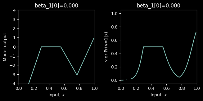
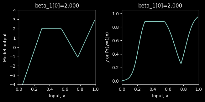
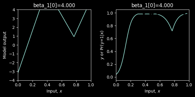
Correct answer = 9.563639387, Your answer = 9.563639387Now let’s investigate finding the maximum likelihood / minimum negative log likelihood solution. For simplicity, we’ll assume that all the parameters are fixed except one and look at how the likelihood and negative log likelihood change as we manipulate the last parameter. We’ll start with overall y_offset, beta_1 (formerly phi_0)
# Define a range of values for the parameter
beta_1_vals = np.arange(-2,6.0,0.1)
# Create some arrays to store the likelihoods, negative log likelihoods
likelihoods = np.zeros_like(beta_1_vals)
nlls = np.zeros_like(beta_1_vals)

# Initialise the parameters
beta_0, omega_0, beta_1, omega_1 = get_parameters()
for count in range(len(beta_1_vals)):
  # Set the value for the parameter
  beta_1[0,0] = beta_1_vals[count]
  # Run the network with new parameters
  model_out = shallow_nn(x_train, beta_0, omega_0, beta_1, omega_1)
  lambda_train = sigmoid(model_out)
  # Compute and store the two values
  likelihoods[count] = compute_likelihood(y_train,lambda_train)
  nlls[count] = compute_negative_log_likelihood(y_train, lambda_train)
  # Draw the model for every 20th parameter setting
  if count % 20 == 0:
    # Run the model to get values to plot and plot it.
    model_out = shallow_nn(x_model, beta_0, omega_0, beta_1, omega_1)
    lambda_model = sigmoid(model_out)
    plot_binary_classification(x_model, model_out, lambda_model, x_train, y_train, title="beta_1[0]=%3.3f"%(beta_1[0,0]))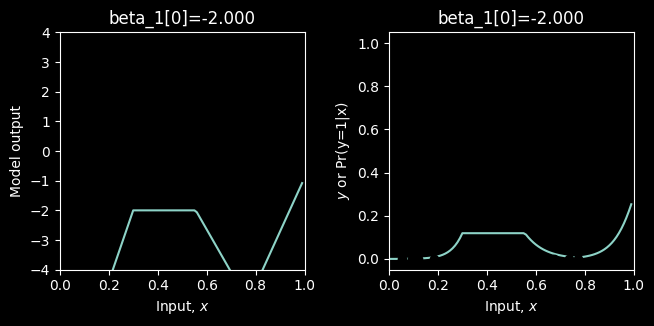
# Now let's plot the likelihood and negative log likelihood as a function of the value of the offset beta1
fig, ax = plt.subplots()
fig.tight_layout(pad=5.0)
likelihood_color = 'tab:red'
nll_color = 'tab:blue'


ax.set_xlabel('beta_1[0]')
ax.set_ylabel('likelihood', color = likelihood_color)
ax.plot(beta_1_vals, likelihoods, color = likelihood_color)
ax.tick_params(axis='y', labelcolor=likelihood_color)

ax1 = ax.twinx()
ax1.plot(beta_1_vals, nlls, color = nll_color)
ax1.set_ylabel('negative log likelihood', color = nll_color)
ax1.tick_params(axis='y', labelcolor = nll_color)

plt.axvline(x = beta_1_vals[np.argmax(likelihoods)], linestyle='dotted')

plt.show()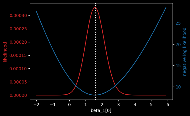
# Hopefully, you can see that the maximum of the likelihood fn is at the same position as the minimum negative log likelihood
# Let's check that:
print("Maximum likelihood = %f, at beta_1=%3.3f"%( (likelihoods[np.argmax(likelihoods)],beta_1_vals[np.argmax(likelihoods)])))
print("Minimum negative log likelihood = %f, at beta_1=%3.3f"%( (nlls[np.argmin(nlls)],beta_1_vals[np.argmin(nlls)])))

# Plot the best model
beta_1[0,0] = beta_1_vals[np.argmin(nlls)]
model_out = shallow_nn(x_model, beta_0, omega_0, beta_1, omega_1)
lambda_model = sigmoid(model_out)
plot_binary_classification(x_model, model_out, lambda_model, x_train, y_train, title="beta_1[0]=%3.3f"%(beta_1[0,0]))
Maximum likelihood = 0.000330, at beta_1=1.600
Minimum negative log likelihood = 8.016513, at beta_1=1.600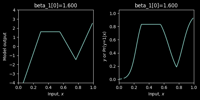
They both give the same answer. But you can see from the likelihood above that the likelihood is very small unless the parameters are almost correct. So in practice, we would work with the negative log likelihood.
Again, to fit the full neural model we would vary all of the 10 parameters of the network in the \(\mathbf{\beta_0, \omega_0, \beta_1, \omega_1}\) until we find the combination that have the maximum likelihood / minimum negative log likelihood.