Backprop for NN

In order for us to see backprop for Neural Networks, we will need some rules of matrix calculus.

Rule of Matrix Calculus:

Derivative of a matrix-vector product: \(\frac{\partial}{\partial \mathbf{x}} (\mathbf{A}\mathbf{x}) = \mathbf{A}^{T}\) here \(\mathbf{A}\) is a matrix and \(\mathbf{x}\) is a vector.
Derivative of a scalar with respect to a vector: \(\frac{\partial}{\partial \mathbf{x}} (\mathbf{a}^{T}\mathbf{x}) = \mathbf{a}\) here \(\mathbf{a}\) is a vector and \(\mathbf{x}\) is a vector.
Derivative of a vector with respect to itself: \(\frac{\partial}{\partial \mathbf{x}} (\mathbf{x}) = \mathbf{I}\) where \(\mathbf{x}\) is a vector and \(\mathbf{I}\) is the identity matrix. An identity matrix has ones on the diagonal and zeros elsewhere.
If \(\mathbf{a}\) is a vector \(\begin{bmatrix} a_1 \\ a_2 \\ a_3 \end{bmatrix}\) then \(\frac{\partial f}{\partial \mathbf{a}} = \begin{bmatrix} \frac{\partial f}{\partial a_1} \\ \frac{\partial f}{\partial a_2} \\ \frac{\partial f}{\partial a_3} \end{bmatrix}\)
If \(\mathbf{A}\) is a matrix \(\mathbf{A} = \begin{bmatrix} a_{11} & a_{12} & a_{13} \\ a_{21} & a_{22} & a_{23} \\ a_{31} & a_{32} & a_{33} \end{bmatrix}\) then \(\frac{\partial f}{\partial \mathbf{A}} = \begin{bmatrix} \frac{\partial f}{\partial a_{11}} & \frac{\partial f}{\partial a_{12}} & \frac{\partial f}{\partial a_{13}} \\ \frac{\partial f}{\partial a_{21}} & \frac{\partial f}{\partial a_{22}} & \frac{\partial f}{\partial a_{23}} \\ \frac{\partial f}{\partial a_{31}} & \frac{\partial f}{\partial a_{32}} & \frac{\partial f}{\partial a_{33}} \end{bmatrix}\)
If \(\mathbf{x}\) is a vector and \(f\) is a scalar function of \(\mathbf{x}\), \(\mathbf{x} = \begin{bmatrix} x_1 \\ x_2 \\ x_3 \end{bmatrix}\) then \(\frac{\partial f}{\partial \mathbf{x}} = \begin{bmatrix} \frac{\partial f}{\partial x_1} \\ \frac{\partial f}{\partial x_2} \\ \frac{\partial f}{\partial x_3} \end{bmatrix}\)
If \(\mathbf{a}\) is a vector and \(f\) is a vector function, \(\mathbf{a} = \begin{bmatrix} a_1 \\ a_2 \\ a_3 \end{bmatrix}\) and \(\mathbf{f} = \begin{bmatrix} f_1 \\ f_2 \\ f_3 \end{bmatrix}\) then \(\frac{\partial \mathbf{f}}{\partial \mathbf{a}} = \begin{bmatrix} \frac{\partial f_1}{\partial a_1} & \frac{\partial f_1}{\partial a_2} & \frac{\partial f_1}{\partial a_3} \\ \frac{\partial f_2}{\partial a_1} & \frac{\partial f_2}{\partial a_2} & \frac{\partial f_2}{\partial a_3} \\ \frac{\partial f_3}{\partial a_1} & \frac{\partial f_3}{\partial a_2} & \frac{\partial f_3}{\partial a_3} \end{bmatrix}\)

Now we run backpropagation for a three-layer network.

Forward pass

We write the network as a series of sequential calculations:

\[\begin{eqnarray} \mathbf{f}_{0} &=& \boldsymbol\beta_{0} +\boldsymbol\Omega_{0}\mathbf{x}_i\nonumber \\ \mathbf{h}_{1} &=& \mathbf{a}[\mathbf{f}_{0}]\nonumber \\ \mathbf{f}_{1} &=& \boldsymbol\beta_{1} +\boldsymbol\Omega_{1}\mathbf{h}_{1}\nonumber \\ \mathbf{h}_{2} &=& \mathbf{a}[\mathbf{f}_{1}]\nonumber \\ \mathbf{f}_{2} &=& \boldsymbol\beta_{2} +\boldsymbol\Omega_{2}\mathbf{h}_{2}\nonumber \\ \mathbf{h}_{3} &=& \mathbf{a}[\mathbf{f}_{2}]\nonumber \\ \mathbf{f}_{3}&=& \boldsymbol\beta_{3} +\boldsymbol\Omega_{3}\mathbf{h}_{3}\nonumber \\ \ell_{i} &=& \mbox{l}[\mathbf{f}_{3},y_{i}], \end{eqnarray}\]

where \(\mathbf{f}_{k-1}\) represents the pre-activations at the \(k^{th}\) hidden layer (i.e., the values before the ReLU function \(\mathbf{a}[\cdot]\)) and \(\mathbf{h}_k\) contains the activations at the \(k^{th}\) hidden layer (i.e., after the ReLU function).

The term \(\mbox{l}[\mathbf{f}_3,y_i]\) represents the loss function (e.g., least squares or binary cross-entropy loss).

In the forward pass, we work through these calculations and store all the intermediate quantities.

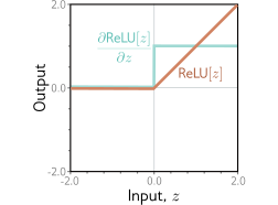
Derivative of rectified linear unit. The rectified linear unit (orange curve) returns zero when the input is less than zero and returns the input otherwise. Its derivative (cyan curve) returns zero when the input is less than zero (since the slope here is zero) and one when the input is greater than zero (since the slope here is one).

Backward pass #1

Now let’s consider how the loss changes when the pre-activations \(\mathbf{f}_0,\mathbf{f}_1,\mathbf{f}_2\) change. Applying the chain rule, the expression for the derivative of the loss \(\ell_{i}\) with respect to \(\mathbf{f}_2\) is:

\[\begin{eqnarray}\label{eq:train2_backward1} \frac{\partial \ell_{i}}{\partial \mathbf{f}_{2}}=\frac{\partial \mathbf{h}_{3}}{\partial \mathbf{f}_{2}}\frac{\partial \mathbf{f}_3}{\partial \mathbf{h}_{3}} \frac{\partial \ell_{i}}{\partial \mathbf{f}_3}. \end{eqnarray}\]

The three terms on the right-hand side have sizes \(\text{D}_3 \times \text{D}_3, \text{D}_3 \times \text{D}_f \text{and } \text{D}_f\times 1\), respectively, where \(D_3\) is the number of hidden units in the third layer, and \(D_f\) is the dimensionality of the model output \(\mathbf{f}_3\).

Similarly, we can compute how the loss changes when we change \(\mathbf{f}_1\) and \(\mathbf{f}_0\):

\[\begin{eqnarray}\label{eq:train2_backward2} \frac{\partial \ell_{i}}{\partial \mathbf{f}_{1}}&=& \frac{\partial \mathbf{h}_{2}}{\partial \mathbf{f}_{1}}\frac{\partial \mathbf{f}_{2}}{\partial \mathbf{h}_{2}} \left(\frac{\partial \mathbf{h}_{3}}{\partial \mathbf{f}_{2}}\frac{\partial \mathbf{f}_3}{\partial \mathbf{h}_{3}} \frac{\partial \ell_{i}}{\partial \mathbf{f}_3}\right) \\ \frac{\partial \ell_{i}}{\partial \mathbf{f}_{0}}&=&\frac{\partial \mathbf{h}_{1}}{\partial \mathbf{f}_{0}}\frac{\partial \mathbf{f}_{1}}{\partial \mathbf{h}_{1}}\left(\frac{\partial \mathbf{h}_{2}}{\partial \mathbf{f}_{1}}\frac{\partial \mathbf{f}_{2}}{\partial \mathbf{h}_{2}} \frac{\partial \mathbf{h}_{3}}{\partial \mathbf{f}_{2}}\frac{\partial \mathbf{f}_3}{\partial \mathbf{h}_{3}} \frac{\partial \ell_{i}}{\partial \mathbf{f}_3}\right).\label{eq:train2_backward2a} \end{eqnarray}\]

Note that in each case, the term in brackets was computed in the previous step. By working backward through the network, we can reuse the previous computations.

Moreover, the terms themselves are simple. Working backward through the right-hand side of equation, we have:

The derivative \(\frac{\partial \ell_{i}}{\partial \mathbf{f}_3}\) of the loss \(\ell_{i}\) with respect to the network output \(\mathbf{f}_3\) will depend on the loss function but usually has a simple form.
The derivative \(\frac{\partial \mathbf{f}_3}{\partial \mathbf{h}_{3}}\) of the network output with respect to hidden layer \(\mathbf{h}_{3}\) is:

\[\begin{eqnarray} \frac{\partial \mathbf{f}_3}{\partial \mathbf{h}_{3}} = \frac{\partial}{\partial \mathbf{h}_{3}}\left(\boldsymbol\beta_{3} +\boldsymbol\Omega_{3}\mathbf{h}_{3}\right) = \boldsymbol\Omega_{3}^{T}. \end{eqnarray}\]

If you are unfamiliar with matrix calculus, this result is not obvious.

The derivative \(\frac{\partial \mathbf{h}_{3}}{\partial \mathbf{f}_{2}}\) of the output \(\mathbf{h}_{3}\) of the activation function with respect to its input \(f_2\) will depend on the activation function. It will be a diagonal matrix since each activation only depends on the corresponding pre-activation. For ReLU since each activation only depends on the corresponding pre-activation. For ReLU functions, the diagonal terms are zero everywhere \(\mathbf{f}_{2}\) is less than \(0\) and one otherwise (figure 7.6). Rather than multiply by this matrix, we extract the diagonal terms as a vector \(\mathbf{I}[\mathbf{f}_{2} >0]\) and pointwise multiply, which is more efficient.

The terms on the right-hand side of equations 7.19 and 7.20 have similar forms. As we progress back through the network, we alternately

multiply by the transpose of the weight matrices \(\boldsymbol\Omega_{k}^{T}\) and
threshold based on the inputs \(\mathbf{f}_{k-1}\) to the hidden layer. These inputs were stored during the forward pass.

Backward Pass # 2

Now that we know how to compute \(\frac{\partial \ell_{i}}{\partial \mathbf{f}_{k}}\), we can focus on calculating the derivatives of the loss with respect to the weights and biases. To calculate the derivatives of the loss with respect to the biases \(\boldsymbol\beta_k\), we again use the chain rule:

\[\begin{eqnarray} \frac{\partial \ell_{i}}{\partial \boldsymbol\beta_k} &=& \frac{\partial \mathbf{f}_{k}}{\partial \boldsymbol\beta_k} \frac{\partial \ell_{i}}{\partial \mathbf{f}_{k}} \nonumber\\ &=& \frac{\partial}{\partial \boldsymbol\beta_k}\left(\boldsymbol\beta_{k} +\boldsymbol\Omega_{k}\mathbf{h}_{k}\right) \frac{\partial \ell_{i}}{\partial \mathbf{f}_{k}} \nonumber \\ &=& \frac{\partial \ell_{i}}{\partial \mathbf{f}_{k}}, \end{eqnarray}\]

which we already calculated in equations 7.18 and 7.19. Similarly, the derivative for the weights matrix \(\boldsymbol\Omega_k\), is given by:

\[\begin{eqnarray} \frac{\partial \ell_{i}}{\partial \boldsymbol\Omega_k} &=& \frac{\partial \mathbf{f}_{k}}{\partial \boldsymbol\Omega_k} \frac{\partial \ell_{i}}{\partial \mathbf{f}_{k}} \nonumber\\ &=& \frac{\partial}{\partial \boldsymbol\Omega_k}\left(\boldsymbol\beta_{k} +\boldsymbol\Omega_{k}\mathbf{h}_{k}\right) \frac{\partial \ell_{i}}{\partial \mathbf{f}_{k}} \nonumber \\ &=& \frac{\partial \ell_{i}}{\partial \mathbf{f}_{k}}\mathbf{h}_k^{T}. \end{eqnarray}\]

Again, the progression from line two to line three is not obvious and is explored in problem 7.9.

However, the result makes sense. The final line is a matrix of the same size as \(\boldsymbol\Omega_k\). It depends linearly on \(\mathbf{h}_k\), which was multiplied by \(\boldsymbol\Omega_k\) in the original expression.

This is also consistent with the initial intuition that the derivative of the weights in \(\boldsymbol\Omega_k\) will be proportional to the values of the hidden units \(\mathbf{h}_k\) that they multiply. Recall that we already computed these during the forward pass.

Summary

We now briefly summarize the final backpropagation algorithm.

Consider a deep neural network \(f[x_i,\boldsymbol\phi]\) that takes input \(x_i\), has \(K\) hidden layers with ReLU activations, and individual loss term \(\ell_i = l[f[x_i,\boldsymbol\phi],y_i]\).

The goal of backpropagation is to compute the derivatives \(\partial \ell_i/\partial \boldsymbol\beta_k\) and \(\partial \ell_i/\partial \boldsymbol\Omega_k\) with respect to the biases \(\boldsymbol\beta_k\) and weights \(\boldsymbol\Omega_k\).

Forward Pass

We compute and store the following quantities:

\[\begin{eqnarray} \mathbf{f}_{0} &=& \boldsymbol\beta_{0} +\boldsymbol\Omega_{0}\mathbf{x}_i\nonumber \\ \mathbf{h}_{k} &=& \mathbf{a}[\mathbf{f}_{k-1}]\hspace{2.76cm} k\in\{1,2,\ldots, K\}\nonumber \\ \mathbf{f}_{k} &=& \boldsymbol\beta_{k} +\boldsymbol\Omega_{k}\mathbf{h}_{k}.\hspace{2cm} k\in\{1,2,\ldots, K\} \end{eqnarray}\]

Backward Pass

We start with the derivative \(\partial \ell_i/\partial \mathbf{f}_K\) of the loss function \(\ell_i\) with respect to the network output \(\mathbf{f}_K\) and work backward through the network:

\[\begin{eqnarray}\label{eq:train2_bp_backward_summary} \frac{\partial \ell_{i}}{\partial \boldsymbol\beta_k} &=& \frac{\partial \ell_{i}}{\partial \mathbf{f}_k} \hspace{4.1cm} k\in\{K,K-1,\ldots, 1\}\nonumber\\ \frac{\partial \ell_{i}}{\partial \boldsymbol\Omega_k} &=& \frac{\partial \ell_{i}}{\partial \mathbf{f}_k}\mathbf{h}_{k}^{T}\hspace{3.65cm} k\in\{K,K-1,\ldots, 1\}\nonumber\\ \frac{\partial \ell_{i}}{\partial \mathbf{f}_{k-1}} &=& \mathbb{I}[\mathbf{f}_{k-1}>0]\odot \left(\boldsymbol\Omega_{k}^{T}\frac{\partial \ell_{i}}{\partial \mathbf{f}_{k}}\right),\hspace{0.82cm} k\in\{K,K-1,\ldots, 1\} \end{eqnarray}\]

where ⊙ denotes pointwise multiplication, and \(\mathbb{I}[\mathbf{f}_{k-1} > 0]\) is a vector containing ones where \(\mathbf{f}_{k-1}\) is greater than zero and zeros elsewhere. Finally, we compute the derivatives with respect to the first set of biases and weights:

\[\begin{eqnarray} \frac{\partial \ell_{i}}{\partial \boldsymbol\beta_0} &=& \frac{\partial \ell_{i}}{\partial \mathbf{f}_0} \nonumber\\ \frac{\partial \ell_{i}}{\partial \boldsymbol\Omega_0} &=& \frac{\partial \ell_{i}}{\partial \mathbf{f}_0}\mathbf{x}_{i}^{T}. \end{eqnarray}\]

We calculate these derivatives for every training example in the batch and sum them together to retrieve the gradient for the SGD update.

Note that the backpropagation algorithm is extremely eﬀicient; the most demanding computational step in both the forward and backward pass is matrix multiplication (by Ω and ΩT , respectively) which only requires additions and multiplications. However, it is not memory eﬀicient; the intermediate values in the forward pass must all be stored, and this can limit the size of the model we can train.

import numpy as np
import matplotlib.pyplot as plt

# Set seed so we always get the same random numbers
np.random.seed(0)

# Number of hidden layers
K   = 5
# Number of neurons per layer
D   = 6
# Input layer
D_i = 1
# Output layer
D_o = 1

# Make empty lists
all_weights     = [None] * (K+1)
all_biases      = [None] * (K+1)

# Create input and output layers
all_weights[0]  = np.random.normal(size=(D, D_i))
all_weights[-1] = np.random.normal(size=(D_o, D))
all_biases[0]   = np.random.normal(size =(D,1))
all_biases[-1]  = np.random.normal(size =(D_o,1))

# Create intermediate layers
for layer in range(1,K):
  all_weights[layer] = np.random.normal(size=(D,D))
  all_biases[layer] = np.random.normal(size=(D,1))
     

# Define the Rectified Linear Unit (ReLU) function
def ReLU(preactivation):
  activation = preactivation.clip(0.0)
  return activation

def compute_network_output(net_input, all_weights, all_biases):

  # Retrieve number of layers
  K = len(all_weights) -1

  # We'll store the pre-activations at each layer in a list "all_f"
  # and the activations in a second list "all_h".
  all_f = [None] * (K+1)
  all_h = [None] * (K+1)

  #For convenience, we'll set
  # all_h[0] to be the input, and all_f[K] will be the output
  all_h[0] = net_input

  # Run through the layers, calculating all_f[0...K-1] and all_h[1...K]
  for layer in range(K):
      # Update preactivations and activations at this layer according to eqn 7.17
      all_f[layer] = np.matmul(all_weights[layer], all_h[layer]) + all_biases[layer]
      all_h[layer+1] = ReLU(all_f[layer])

  # Compute the output from the last hidden layer
  all_f[K] = np.matmul(all_weights[K], all_h[K]) + all_biases[K]

  # Retrieve the output
  net_output = all_f[K]

  return net_output, all_f, all_h

# Define input
net_input = np.ones((D_i,1)) * 1.2
# Compute network output
net_output, all_f, all_h = compute_network_output(net_input,all_weights, all_biases)
print("True output = %3.3f, Your answer = %3.3f"%(1.907, net_output[0,0]))

True output = 1.907, Your answer = 1.907

def least_squares_loss(net_output, y):
  return np.sum((net_output-y) * (net_output-y))

def d_loss_d_output(net_output, y):
    return 2*(net_output -y);
     

y = np.ones((D_o,1)) * 20.0
loss = least_squares_loss(net_output, y)
print("y = %3.3f Loss = %3.3f"%(y, loss))

y = 20.000 Loss = 327.371

# We'll need the indicator function
def indicator_function(x):
  x_in = np.array(x)
  x_in[x_in>0] = 1
  x_in[x_in<=0] = 0
  return x_in

# Main backward pass routine
def backward_pass(all_weights, all_biases, all_f, all_h, y):
  all_dl_dweights           = [None] * (K+1)
  all_dl_dbiases            = [None] * (K+1)
  all_dl_df                 = [None] * (K+1)
  all_dl_dh                 = [None] * (K+1)
  all_dl_df[K]              = np.array(d_loss_d_output(all_f[K],y))
  for layer in range(K,-1,-1):
    all_dl_dbiases[layer]   = np.array(all_dl_df[layer])
    all_dl_dweights[layer]  = np.array(all_dl_df[layer]) @ all_h[layer].T
    all_dl_dh[layer]        = all_weights[layer].T @ all_dl_df[layer]
    if layer > 0:
      all_dl_df[layer-1]    = all_dl_dh[layer] * indicator_function(all_f[layer-1])
  return all_dl_dweights, all_dl_dbiases
     

all_dl_dweights, all_dl_dbiases = backward_pass(all_weights, all_biases, all_f, all_h, y)
    
np.set_printoptions(precision=3)
# Make space for derivatives computed by finite differences
all_dl_dweights_fd  = [None] * (K+1)
all_dl_dbiases_fd   = [None] * (K+1)

# Let's test if we have the derivatives right using finite differences
delta_fd            = 0.000001

# Test the dervatives of the bias vectors
for layer in range(K+1):
  dl_dbias  = np.zeros_like(all_dl_dbiases[layer])
  # For every element in the bias
  for row in range(all_biases[layer].shape[0]):
    # Take copy of biases  We'll change one element each time
    all_biases_copy              = [np.array(x) for x in all_biases]
    all_biases_copy[layer][row] += delta_fd
    network_output_1, *_         = compute_network_output(net_input, all_weights, all_biases_copy)
    network_output_2, *_         = compute_network_output(net_input, all_weights, all_biases)
    dl_dbias[row] = (least_squares_loss(network_output_1, y) - least_squares_loss(network_output_2,y))/delta_fd
  
  all_dl_dbiases_fd[layer] = np.array(dl_dbias)
  print("-----------------------------------------------")
  print("Bias %d, derivatives from backprop:"%(layer))
  print(all_dl_dbiases[layer])
  print("Bias %d, derivatives from finite differences"%(layer))
  print(all_dl_dbiases_fd[layer])
  if np.allclose(all_dl_dbiases_fd[layer],all_dl_dbiases[layer],rtol=1e-05, atol=1e-08, equal_nan=False):
    print("Success!  Derivatives match.")
  else:
    print("Failure!  Derivatives different.")



# Test the derivatives of the weights matrices
for layer in range(K+1):
  dl_dweight  = np.zeros_like(all_dl_dweights[layer])
  # For every element in the bias
  for row in range(all_weights[layer].shape[0]):
    for col in range(all_weights[layer].shape[1]):
      # Take copy of biases  We'll change one element each time
      all_weights_copy = [np.array(x) for x in all_weights]
      all_weights_copy[layer][row][col] += delta_fd
      network_output_1, *_ = compute_network_output(net_input, all_weights_copy, all_biases)
      network_output_2, *_ = compute_network_output(net_input, all_weights, all_biases)
      dl_dweight[row][col] = (least_squares_loss(network_output_1, y) - least_squares_loss(network_output_2,y))/delta_fd
  
  all_dl_dweights_fd[layer] = np.array(dl_dweight)
  print("-----------------------------------------------")
  print("Weight %d, derivatives from backprop:"%(layer))
  print(all_dl_dweights[layer])
  print("Weight %d, derivatives from finite differences"%(layer))
  print(all_dl_dweights_fd[layer])
  if np.allclose(all_dl_dweights_fd[layer],all_dl_dweights[layer],rtol=1e-05, atol=1e-08, equal_nan=False):
    print("Success!  Derivatives match.")
  else:
    print("Failure!  Derivatives different.")

-----------------------------------------------
Bias 0, derivatives from backprop:
[[ -4.486]
 [  4.947]
 [  6.812]
 [ -3.883]
 [-24.935]
 [  0.   ]]
Bias 0, derivatives from finite differences
[[ -4.486]
 [  4.947]
 [  6.812]
 [ -3.883]
 [-24.935]
 [  0.   ]]
Success!  Derivatives match.
-----------------------------------------------
Bias 1, derivatives from backprop:
[[ -0.   ]
 [-11.297]
 [  0.   ]
 [  0.   ]
 [-10.722]
 [  0.   ]]
Bias 1, derivatives from finite differences
[[  0.   ]
 [-11.297]
 [  0.   ]
 [  0.   ]
 [-10.722]
 [  0.   ]]
Success!  Derivatives match.
-----------------------------------------------
Bias 2, derivatives from backprop:
[[-0.   ]
 [-0.   ]
 [ 0.938]
 [ 0.   ]
 [-9.993]
 [ 0.508]]
Bias 2, derivatives from finite differences
[[ 0.   ]
 [ 0.   ]
 [ 0.938]
 [ 0.   ]
 [-9.993]
 [ 0.508]]
Success!  Derivatives match.
-----------------------------------------------
Bias 3, derivatives from backprop:
[[-0.   ]
 [-4.8  ]
 [-1.661]
 [-0.   ]
 [ 3.393]
 [ 5.391]]
Bias 3, derivatives from finite differences
[[ 0.   ]
 [-4.8  ]
 [-1.661]
 [ 0.   ]
 [ 3.393]
 [ 5.391]]
Success!  Derivatives match.
-----------------------------------------------
Bias 4, derivatives from backprop:
[[-0.   ]
 [ 0.   ]
 [ 0.   ]
 [-0.   ]
 [-5.212]
 [-0.   ]]
Bias 4, derivatives from finite differences
[[ 0.   ]
 [ 0.   ]
 [ 0.   ]
 [ 0.   ]
 [-5.212]
 [ 0.   ]]
Success!  Derivatives match.
-----------------------------------------------
Bias 5, derivatives from backprop:
[[-36.187]]
Bias 5, derivatives from finite differences
[[-36.187]]
Success!  Derivatives match.
-----------------------------------------------
Weight 0, derivatives from backprop:
[[ -5.383]
 [  5.937]
 [  8.174]
 [ -4.66 ]
 [-29.922]
 [  0.   ]]
Weight 0, derivatives from finite differences
[[ -5.383]
 [  5.937]
 [  8.174]
 [ -4.66 ]
 [-29.922]
 [  0.   ]]
Success!  Derivatives match.
-----------------------------------------------
Weight 1, derivatives from backprop:
[[  0.      0.      0.      0.      0.      0.   ]
 [-32.511  -6.799 -18.282 -34.148 -42.196   0.   ]
 [  0.      0.      0.      0.      0.      0.   ]
 [  0.      0.      0.      0.      0.      0.   ]
 [-30.856  -6.453 -17.352 -32.409 -40.047   0.   ]
 [  0.      0.      0.      0.      0.      0.   ]]
Weight 1, derivatives from finite differences
[[  0.      0.      0.      0.      0.      0.   ]
 [-32.511  -6.799 -18.282 -34.148 -42.196   0.   ]
 [  0.      0.      0.      0.      0.      0.   ]
 [  0.      0.      0.      0.      0.      0.   ]
 [-30.856  -6.453 -17.352 -32.409 -40.047   0.   ]
 [  0.      0.      0.      0.      0.      0.   ]]
Success!  Derivatives match.
-----------------------------------------------
Weight 2, derivatives from backprop:
[[  0.      0.      0.      0.      0.      0.   ]
 [  0.      0.      0.      0.      0.      0.   ]
 [  0.      5.371   0.      0.      3.145   0.   ]
 [  0.      0.      0.      0.      0.      0.   ]
 [  0.    -57.233   0.      0.    -33.506   0.   ]
 [  0.      2.907   0.      0.      1.702   0.   ]]
Weight 2, derivatives from finite differences
[[  0.      0.      0.      0.      0.      0.   ]
 [  0.      0.      0.      0.      0.      0.   ]
 [  0.      5.371   0.      0.      3.145   0.   ]
 [  0.      0.      0.      0.      0.      0.   ]
 [  0.    -57.233   0.      0.    -33.506   0.   ]
 [  0.      2.907   0.      0.      1.702   0.   ]]
Success!  Derivatives match.
-----------------------------------------------
Weight 3, derivatives from backprop:
[[  0.      0.      0.      0.      0.      0.   ]
 [  0.      0.     -3.674   0.    -42.905 -10.998]
 [  0.      0.     -1.272   0.    -14.85   -3.807]
 [  0.      0.      0.      0.      0.      0.   ]
 [  0.      0.      2.597   0.     30.333   7.776]
 [  0.      0.      4.126   0.     48.188  12.353]]
Weight 3, derivatives from finite differences
[[  0.      0.      0.      0.      0.      0.   ]
 [  0.      0.     -3.674   0.    -42.905 -10.998]
 [  0.      0.     -1.272   0.    -14.85   -3.807]
 [  0.      0.      0.      0.      0.      0.   ]
 [  0.      0.      2.597   0.     30.333   7.776]
 [  0.      0.      4.126   0.     48.188  12.353]]
Success!  Derivatives match.
-----------------------------------------------
Weight 4, derivatives from backprop:
[[  0.      0.      0.      0.      0.      0.   ]
 [  0.      0.      0.      0.      0.      0.   ]
 [  0.      0.      0.      0.      0.      0.   ]
 [  0.      0.      0.      0.      0.      0.   ]
 [  0.    -81.635 -49.136   0.    -22.007 -10.146]
 [  0.      0.      0.      0.      0.      0.   ]]
Weight 4, derivatives from finite differences
[[  0.      0.      0.      0.      0.      0.   ]
 [  0.      0.      0.      0.      0.      0.   ]
 [  0.      0.      0.      0.      0.      0.   ]
 [  0.      0.      0.      0.      0.      0.   ]
 [  0.    -81.635 -49.136   0.    -22.007 -10.146]
 [  0.      0.      0.      0.      0.      0.   ]]
Success!  Derivatives match.
-----------------------------------------------
Weight 5, derivatives from backprop:
[[   0.      0.      0.      0.   -400.33    0.  ]]
Weight 5, derivatives from finite differences
[[   0.      0.      0.      0.   -400.33    0.  ]]
Success!  Derivatives match.