import numpy as np
import matplotlib.pyplot as plt

def init_params(K, D, sigma_sq_omega):
  # Set seed so we always get the same random numbers
  np.random.seed(0)

  # Input layer
  D_i = 1
  # Output layer
  D_o = 1

  # Make empty lists
  all_weights = [None] * (K+1)
  all_biases = [None] * (K+1)

  # Create input and output layers
  all_weights[0] = np.random.normal(size=(D, D_i))*np.sqrt(sigma_sq_omega)
  all_weights[-1] = np.random.normal(size=(D_o, D)) * np.sqrt(sigma_sq_omega)
  all_biases[0] = np.zeros((D,1))
  all_biases[-1]= np.zeros((D_o,1))

  # Create intermediate layers
  for layer in range(1,K):
    all_weights[layer] = np.random.normal(size=(D,D))*np.sqrt(sigma_sq_omega)
    all_biases[layer] = np.zeros((D,1))

  return all_weights, all_biases


# Define the Rectified Linear Unit (ReLU) function
def ReLU(preactivation):
  activation = preactivation.clip(0.0)
  return activation


def compute_network_output(net_input, all_weights, all_biases):

  # Retrieve number of layers
  K = len(all_weights)-1

  # We'll store the pre-activations at each layer in a list "all_f"
  # and the activations in a second list "all_h".
  all_f = [None] * (K+1)
  all_h = [None] * (K+1)

  #For convenience, we'll set
  # all_h[0] to be the input, and all_f[K] will be the output
  all_h[0] = net_input

  # Run through the layers, calculating all_f[0...K-1] and all_h[1...K]
  for layer in range(K):
      # Update preactivations and activations at this layer according to eqn 7.5
      all_f[layer] = all_biases[layer] + np.matmul(all_weights[layer], all_h[layer])
      all_h[layer+1] = ReLU(all_f[layer])

  # Compute the output from the last hidden layer
  all_f[K] = all_biases[K] + np.matmul(all_weights[K], all_h[K])

  # Retrieve the output
  net_output = all_f[K]

return net_output, all_f, all_hParameter Initialization
The backpropagation algorithm computes the derivatives that are used by stochastic gradient descent and Adam to train the model.
We now address how to initialize the parameters before we start training.
To see why this is crucial, consider that during the forward pass, each set of pre-activations \(\mathbf{f}_k\) is computed as:
\[\begin{eqnarray} \mathbf{f}_{k} &=& \boldsymbol\beta_{k} +\boldsymbol\Omega_{k}\mathbf{h}_{k}\nonumber\\ &=& \boldsymbol\beta_{k} +\boldsymbol\Omega_{k}\textbf{a}[\mathbf{f}_{k-1}], \end{eqnarray}\]
where a[•] applies the ReLU functions and matrices \(\Omega_k\) and vectors \(\boldsymbol\beta_k\) are the weights and biases, respectively.
Imagine that we initialize all the biases to zero and the elements of \(\Omega_k\) according to a normal distribution with mean zero and variance \(\sigma^2\).
Consider two scenarios:
Vanishing Gradient Problem
If the variance \(\sigma^2\) is very small (e.g., \(10^{-5}\)), then each element of \(\beta_k + \Omega_k \mathbf{h}_k\) will be a weighted sum of \(\mathbf{h}_k\) where the weights are very small.
The result will likely have a smaller magnitude than the input. In addition, the ReLU function clips values less than zero, so the range of \(\mathbf{h}_k\) will be half that of \(\mathbf{f}_{k-1}\). Consequently, the magnitudes of the pre-activations at the hidden layers will get smaller and smaller as we progress through the network.
Exploding Gradient Problem
If the variance \(\sigma^2\) is very large (e.g., \(10^5\)), then each element of \(\beta_k + \Omega_k \mathbf{h}_k\) will be a weighted sum of \(\mathbf{h}_k\) where the weights are very large. The result is likely to have a much larger magnitude than the input.
The ReLU function halves the range of the inputs, but if \(\sigma^2\) is large enough, the magnitudes of the pre-activations will still get larger as we progress through the network.
In these two situations, the values at the pre-activations can become so small or so large that they cannot be represented with finite precision floating point arithmetic.
Even if the forward pass is tractable, the same logic applies to the backward pass.
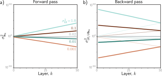
Consider a deep network with 50 hidden layers and \(D_h = 100\) hidden units per layer.
The network has a 100-dimensional input \(x\) initialized from a standard normal distribution, a single fixed target y = 0, and the bias vectors \(\beta_k\) are initialized to zero, and the weight matrices \(\Omega_k\) are initialized with a normal distribution \(\mathcal{N}(0, \sigma^2_\Omega)\) with mean zero and five different variances \(\sigma^2_\Omega\) \(\in \{0.001, 0.01, 0.02, 0.1, 1.0\}\).
Variance of hidden unit activations computed in forward pass as a function of the network layer. For He initialization (\(\sigma^2_\Omega = 2/_h = 0.02\)), the variance is stable. However, for larger values, it increases rapidly, and for smaller values, it decreases rapidly (note log scale).
The variance of the gradients in the backward pass (solid lines) continues this trend; if we initialize with a value larger than 0.02, the magnitude of the gradients increases rapidly as we pass back through the network. If we initialize with a value smaller, then the magnitude decreases. These are known as the exploding gradient and vanishing gradient problems, respectively.
In the equation,
\[\begin{eqnarray} \mathbf{h}_{k} &=& \textbf{a}[\boldsymbol\beta_{k-1} +\boldsymbol\Omega_{k-1}\mathbf{h}_{k-1}]\nonumber\\ \end{eqnarray}\]
\(\boldsymbol\Omega_{k-1}\mathbf{h}_{k-1}\) unpack as \(\sum_{j=1}^{D_h} \Omega_{k-1,ij} h_{k-1,j}\) for each element \(i\) of the resulting vector.
Because we are adding \(D_h\) terms in the sum, the variance of each element of \(\boldsymbol\Omega_{k-1}\mathbf{h}_{k-1}\) will scale with \(D_h\).
In other words, variance of \(\text{variance}(\mathbf{h}_{k}) \approx D_h \text{variance}(h_{k-1})\) will also scale with \(D_h\) if we do not adjust the initialization of the weights.
The goal is to have variance of \(\mathbf{h}_{k} \approx \mathbf{h}_{k-1}\) remain relatively constant as we propagate through the layers.
Roughly speaking, if \(\boldsymbol\beta_{k-1} +\boldsymbol\Omega_{k-1}\mathbf{h}_{k-1}\) is symmetrically distributed around zero, ReLU kills half of the values:
He Initialization
Initialization for forward pass
We now present a mathematical version of the same argument. Consider the computation between adjacent pre-activations \(f\) and \(f ′\) with dimensions \(D_h\) and \(D_h′\), respectively:
\[\begin{eqnarray} \mathbf{h} &=& \mbox{\bf a}[\mathbf{f}],\nonumber \\ \mathbf{f}' &=& \boldsymbol\beta +\boldsymbol\Omega\mathbf{h} \end{eqnarray}\]
where \(h\) represents the activations, \(\Omega\) and \(\beta\) represent the weights and biases, and a[•] is the activation function.
Assume the pre-activations \(f_j\) in the input layer \(f\) have variance \(\sigma^2_f\). Consider initializing the biases \(\beta_i\) to zero and the weights \(\Omega_{ij}\) as normally distributed with mean zero and variance \(\sigma^2_\Omega\). Now we derive expressions for the mean and variance of the pre-activations \(f ′\) in the subsequent layer.
The expectation (mean) \(\mathbb{E}[f'_{i}]\) of the intermediate values \(f'_{i}\) is:
\[\begin{eqnarray} \mathbb{E}[f'_{i}] &=& \mathbb{E}\left[\beta_{i} + \sum_{j=1}^{D_h}\Omega_{ij}h_{j}\right]\nonumber \\ &=& \mathbb{E}\left[\beta_{i}\right] +\sum_{j=1}^{D_h}\mathbb{E}\left[\Omega_{ij}h_{j}\right] \nonumber\\ &=& \mathbb{E}\left[\beta_{i}\right] +\sum_{j=1}^{D_h}\mathbb{E}\left[\Omega_{ij}\right]\mathbb{E}\left[h_{j}\right] \nonumber\\ &=& 0 + \sum_{j=1}^{D_h} 0\cdot\mathbb{E}\left[h_{j}\right] = 0, \end{eqnarray}\]
where \(D_h\) is the dimensionality of the input layer \(h\). We have used the rules for manipu- lating expectations, and we have assumed that the distributions over the hidden units \(h_j\) and the network weights \(\Omega_{ij}\) are independent between the second and third lines. Using this result, we see that the variance \(\sigma^2_{f ′}\) of the pre-activations \(f′_{i}\) is
\[\begin{eqnarray} \sigma^{2}_{f'_i} &=& \mathbb{E}[f_{i}^{\prime 2}]-\mathbb{E}[f'_{i}]^{2} \nonumber \\ &=& \mathbb{E}\left[\left(\beta_{i}+\sum_{j=1}^{D_h}\Omega_{ij}h_{j}\right)^2\right]-0\nonumber\\ &=& \mathbb{E}\left[\left(\sum_{j=1}^{D_h}\Omega_{ij}h_{j}\right)^2\right]\nonumber\\ &=& \sum_{j=1}^{D_h}\mathbb{E}\left[\Omega_{ij}^2\right]\mathbb{E}\left[h_{j}^2\right]\nonumber \\ &=&\sum_{j=1}^{D_h} \sigma_\Omega^2 \mathbb{E}\left[h_{j}^2\right] = \sigma_\Omega^2 \sum_{j=1}^{D_h} \mathbb{E}\left[h_{j}^2\right], \end{eqnarray}\]
where we have used the variance identity \(\sigma^2 = \mathbb{E}[(z-\mathbb{E}[z])^2] = \mathbb{E}[z^2]-\mathbb{E}[z]^2\). We have assumed once more that the distributions of the weights \(\Omega_{ij}\) and the hidden units \(h_j\) are independent between lines three and four.
Assuming that the distribution of pre-activations \(f_j\) at the previous layer is symmetric about zero, half of these pre-activations will be clipped by the ReLU function, and the second moment \(\mathbb{E}[h_j^2]\) will be half the variance \(\sigma^2_{f}\) of \(f_j\) (see problem 7.14):
\[\begin{eqnarray} \sigma^{2}_{f'_{i}} = \sigma_\Omega^2 \sum_{j=1}^{D_h} \frac{\sigma_{f}^2}{2} = \frac{1}{2}D_{h} \sigma_\Omega^2 \sigma_{f}^2. \end{eqnarray}\]
This, in turn, implies that if we want the variance \(\sigma^2_{f'}\) of the subsequent pre-activations \(f'\) to be the same as the variance \(\sigma^2_{f}\) of the original pre-activations \(f\) during the forward pass, we should set:
\[\begin{eqnarray}\label{eq:train2_init_forward} \sigma_\Omega^2 = \frac{2}{D_h}, \end{eqnarray}\]
where \(D_h\) is the dimension of the original layer to which the weights were applied. This is known as He initialization.
Initialization for backward pass
A similar argument establishes how the variance of the gradients ∂l/∂fk changes during the backward pass. During the backward pass, we multiply by the transpose ΩT of the weight matrix (equation 7.25), so the equivalent expression becomes:
\[\begin{eqnarray}\label{eq:train2_init_back} \sigma_\Omega^2 = \frac{2}{D_{h'}}, \end{eqnarray}\]
where Dh′ is the dimension of the layer that the weights feed into.
Initialization for both forward and backward pass
If the weight matrix Ω is not square (i.e., there are different numbers of hidden units in the two adjacent layers, so Dh and Dh′ differ), then it is not possible to choose the variance to satisfy both equations 7.32 and 7.33 simultaneously. One possible compromise is to use the mean (Dh + Dh′ )/2 as a proxy for the number of terms, which gives:
\[\begin{eqnarray} \sigma_\Omega^2 = \frac{4}{D_{h}+D_{h'}}. \end{eqnarray}\]
Figure 7.7 shows empirically that both the variance of the hidden units in the forward pass and the variance of the gradients in the backward pass remain stable when the parameters are initialized appropriately.
# Number of layers
K = 5
# Number of neurons per layer
D = 8
# Input layer
D_i = 1
# Output layer
D_o = 1
# Set variance of initial weights to 1
sigma_sq_omega = 1.0
# Initialize parameters
all_weights, all_biases = init_params(K,D,sigma_sq_omega)

n_data = 1000
data_in = np.random.normal(size=(1,n_data))
net_output, all_f, all_h = compute_network_output(data_in, all_weights, all_biases)

for layer in range(1,K+1):
  print("Layer %d, std of hidden units = %3.3f"%(layer, np.std(all_h[layer])))


# You can see that the values of the hidden units are increasing on average (the variance is across all hidden units at the layer
# and the 1000 training examples

# TODO
# Change this to 50 layers with 80 hidden units per layer

# TODO
# Now experiment with sigma_sq_omega to try to stop the variance of the forward computation exploding
Layer 1, std of hidden units = 0.811
Layer 2, std of hidden units = 1.472
Layer 3, std of hidden units = 4.547
Layer 4, std of hidden units = 8.896
Layer 5, std of hidden units = 10.106def least_squares_loss(net_output, y):
return np.sum((net_output-y) * (net_output-y))
def d_loss_d_output(net_output, y):
return 2*(net_output -y);
# We'll need the indicator function
def indicator_function(x):
  x_in = np.array(x)
  x_in[x_in>=0] = 1
  x_in[x_in<0] = 0
  return x_in

# Main backward pass routine
def backward_pass(all_weights, all_biases, all_f, all_h, y):
  # Retrieve number of layers
  K = len(all_weights) - 1

  # We'll store the derivatives dl_dweights and dl_dbiases in lists as well
  all_dl_dweights = [None] * (K+1)
  all_dl_dbiases = [None] * (K+1)
  # And we'll store the derivatives of the loss with respect to the activation and preactivations in lists
  all_dl_df = [None] * (K+1)
  all_dl_dh = [None] * (K+1)
  # Again for convenience we'll stick with the convention that all_h[0] is the net input and all_f[k] in the net output

  # Compute derivatives of net output with respect to loss
  all_dl_df[K] = np.array(d_loss_d_output(all_f[K],y))

  # Now work backwards through the network
  for layer in range(K,-1,-1):
    # Calculate the derivatives of biases at layer from all_dl_df[K]. (eq 7.13, line 1)
    all_dl_dbiases[layer] = np.array(all_dl_df[layer])
    # Calculate the derivatives of weight at layer from all_dl_df[K] and all_h[K] (eq 7.13, line 2)
    all_dl_dweights[layer] = np.matmul(all_dl_df[layer], all_h[layer].transpose())

    # Calculate the derivatives of activations from weight and derivatives of next preactivations (eq 7.13, line 3 second part)
    all_dl_dh[layer] = np.matmul(all_weights[layer].transpose(), all_dl_df[layer])
    # Calculate the derivatives of the pre-activation f with respect to activation h (eq 7.13, line 3, first part)
    if layer > 0:
      all_dl_df[layer-1] = indicator_function(all_f[layer-1]) * all_dl_dh[layer]

  return all_dl_dweights, all_dl_dbiases, all_dl_dh, all_dl_df
# Number of layers
K = 5
# Number of neurons per layer
D = 8
# Input layer
D_i = 1
# Output layer
D_o = 1
# Set variance of initial weights to 1
sigma_sq_omega = 1.0
# Initialize parameters
all_weights, all_biases = init_params(K,D,sigma_sq_omega)
# For simplicity we'll just consider the gradients of the weights and biases between the first and last hidden layer
n_data = 100
aggregate_dl_df = [None] * (K+1)
for layer in range(1,K):
# These 3D arrays will store the gradients for every data point
aggregate_dl_df[layer] = np.zeros((D,n_data))
# We'll have to compute the derivatives of the parameters for each data point separately
for c_data in range(n_data):
data_in = np.random.normal(size=(1,1))
y = np.zeros((1,1))
net_output, all_f, all_h = compute_network_output(data_in, all_weights, all_biases)
all_dl_dweights, all_dl_dbiases, all_dl_dh, all_dl_df = backward_pass(all_weights, all_biases, all_f, all_h, y)
for layer in range(1,K):
aggregate_dl_df[layer][:,c_data] = np.squeeze(all_dl_df[layer])
for layer in reversed(range(1,K)):
print("Layer %d, std of dl_dh = %3.3f"%(layer, np.std(aggregate_dl_df[layer].ravel())))
# You can see that the gradients of the hidden units are increasing on average (the standard deviation is across all hidden units at the layer
# and the 100 training examples
# TODO
# Change this to 50 layers with 80 hidden units per layer
# TODO
# Now experiment with sigma_sq_omega to try to stop the variance of the gradients explodingLayer 4, std of dl_dh = 56.472
Layer 3, std of dl_dh = 109.132
Layer 2, std of dl_dh = 340.657
Layer 1, std of dl_dh = 446.654