Gradient Descent

Slides

To fit a model, we need a training set \({x_i,y_i}_{i=1}^{I}\) of input/output pairs. We seek parameters \(\boldsymbol\phi\) for the model \(f[x_i,\boldsymbol\phi]\) that map the inputs \(x_i\) to the outputs \(y_i\) as closely as possible.

To this end, we define a loss function \(L[\boldsymbol\phi]\) that returns a single number that quantifies the mismatch in this mapping. The goal of an optimization algorithm is to find parameters \(\hat{\boldsymbol\phi}\) that minimize the loss:

\[\begin{eqnarray} \hat{\boldsymbol\phi} = \mathop{\rm argmin}_{\boldsymbol\phi}\Bigl[L[\boldsymbol\phi]\Bigr]. \end{eqnarray}\]

There are many families of optimization algorithms, but the standard methods for training neural networks are iterative. These algorithms initialize the parameters heuristically and then adjust them repeatedly in such a way that the loss decreases.The simplest method in this class is gradient descent.

This starts with initial parameters \(\boldsymbol\phi= [\phi_0,\phi_1,...,\phi_N]^T\) and iterates two steps:

Step 1. Compute the derivatives of the loss with respect to the parameters:

\[\begin{eqnarray} \frac{\partial L}{\partial \boldsymbol\phi} = \begin{bmatrix}\frac{\partial L}{\partial \phi_{0}} \\[5pt] \frac{\partial L}{\partial \phi_{1}}\\ \vdots \\[5pt] \frac{\partial L}{\partial \phi_{N}}\end{bmatrix}. \end{eqnarray}\]

Step 2. Update the parameters according to the rule:

\[\begin{eqnarray}\label{eq:train_gradient_descent} \boldsymbol\phi\longleftarrow\boldsymbol\phi - \alpha \cdot \frac{\partial L}{\partial \boldsymbol\phi}, \end{eqnarray}\]

where the positive scalar \(\alpha\) determines the magnitude of the change.

The first step computes the gradient of the loss function at the current position. This determines the uphill direction of the loss function.

The second step moves a small distance \(\alpha\) downhill (hence the negative sign). The parameter \(\alpha\) may be fixed (in which case, we call it a learning rate), or we may perform a line search where we try several values of \(\alpha\) to find the one that most decreases the loss.

At the minimum of the loss function, the surface must be flat (or we could improve further by going downhill). Hence, the gradient will be zero, and the parameters will stop changing. In practice, we monitor the gradient magnitude and terminate the algorithm when it becomes too small.

Linear regression example

Consider applying gradient descent to the 1D linear regression model. The model \(f[x,\phi]\) maps a scalar input xto a scalar output yand has parameters \(ϕ= [\phi_0,\phi1_1]^T\), which represent the y-intercept and the slope:

\[\begin{eqnarray} y &=& \mbox{f}[x,\boldsymbol\phi]\nonumber \\ &=& \phi_{0} + \phi_{1}x. \end{eqnarray}\]

Given a dataset \(\{x_i,y_i\}_{i=1}^{I}\) containing \(I\) input/output pairs, we choose the least squares loss function:

\[\begin{eqnarray}\label{eq:train_lr_cost_function} L[\boldsymbol\phi] \hspace{0.2cm}= \hspace{0.2cm}\sum_{i=1}^{I} \ell_{i} &=& \sum_{i=1}^{I} \left(\mbox{f}[x_i,\boldsymbol\phi]-y_{i}\right)^{2}\nonumber \\ &=& \sum_{i=1}^{I} \left(\phi_{0}+\phi_{1}x_{i}-y_{i}\right)^{2}, \end{eqnarray}\]

where the term \(l_i = (\phi_0 + \phi_1 x_i - y_i)^2\) is the individual contribution to the loss from the \(i^th\) training example.

The derivative of the loss function with respect to the parameters can be decomposed into the sum of the derivatives of the individual contributions:

\[\begin{eqnarray}\label{eq:train_linear_deriv1} \frac{\partial L}{\partial \boldsymbol\phi} = \frac{\partial}{\partial \boldsymbol\phi}\sum_{i=1}^{I} \ell_{i} = \sum_{i=1}^{I} \frac{\partial \ell_{i}}{\partial \boldsymbol\phi}, \end{eqnarray}\]

where these are given by:

\[\begin{eqnarray}\label{eq:train_linear_deriv2} \frac{\partial \ell_{i}}{\partial \boldsymbol\phi} = \begin{bmatrix}\frac{\partial \ell_{i}}{\partial \phi_{0}}\\\\\frac{\partial \ell_{i}}{\partial \phi_{1}}\end{bmatrix} = \begin{bmatrix}2(\phi_{0}+\phi_{1}x_{i}-y_{i})\\ \\ 2x_{i}(\phi_{0}+\phi_{1}x_{i}-y_{i})\end{bmatrix}. \end{eqnarray}\]

We want to determine how the loss changes with respect to each parameter:

\[\frac{\partial L}{\partial \phi_0} \qquad \text{and} \qquad \frac{\partial L}{\partial \phi_1} \]

Start by taking the partial derivative of the loss with respect to (_0):

\[ \frac{\partial L}{\partial \phi_0} = \frac{1}{I} \sum_{i=1}^{I} \frac{\partial}{\partial\phi_0} \left(y_i-\phi_0-\phi_1x_i\right)^2 \]

Apply the chain rule. The derivative of the outer squared term gives \(2(y_i-\phi_0-\phi_1x_i)\):

\[\frac{\partial L}{\partial \phi_0} = \frac{1}{I} \sum_{i=1}^{I} 2\left(y_i-\phi_0-\phi_1x_i\right) \frac{\partial}{\partial\phi_0} \left(y_i-\phi_0-\phi_1x_i\right)\]

Now take the derivative of the inner expression with respect to \(\phi_0\):

\[ \frac{\partial}{\partial\phi_0} \left(y_i-\phi_0-\phi_1x_i\right) = -1 \]

Substituting this back in gives:

\[ \frac{\partial L}{\partial\phi_0} = \frac{1}{I} \sum_{i=1}^{I} 2\left(y_i-\phi_0-\phi_1x_i\right)(-1) \]

Therefore:

\[ \boxed{ \frac{\partial L}{\partial\phi_0} = -\frac{2}{I} \sum_{i=1}^{I} \left(y_i-\hat{y}_i\right) } \]

Equivalently, we can reverse the subtraction and remove the negative sign:

\[ \boxed{ \frac{\partial L}{\partial\phi_0} = \frac{2}{I} \sum_{i=1}^{I} \left(\hat{y}_i-y_i\right) } \]

So the gradient for \(\phi_0\) is essentially the average prediction error, multiplied by 2.

Now do exactly the same thing for \(\phi_1\):

\[ \frac{\partial L}{\partial \phi_1} = \frac{1}{I} \sum_{i=1}^{I} \frac{\partial}{\partial\phi_1} \left(y_i-\phi_0-\phi_1x_i\right)^2 \]

Again, apply the chain rule:

\[ \frac{\partial L}{\partial \phi_1} = \frac{1}{I} \sum_{i=1}^{I} 2\left(y_i-\phi_0-\phi_1x_i\right) \frac{\partial}{\partial\phi_1} \left(y_i-\phi_0-\phi_1x_i\right) \]

This time, the derivative of the inner expression is different. With respect to \(\phi_1\):

\[ \frac{\partial}{\partial\phi_1} \left(y_i-\phi_0-\phi_1x_i\right) = -x_i \]

Substitute that into the derivative:

\[ \frac{\partial L}{\partial\phi_1} = \frac{1}{I} \sum_{i=1}^{I} 2\left(y_i-\phi_0-\phi_1x_i\right)(-x_i) \]

Therefore:

\[ \boxed{ \frac{\partial L}{\partial\phi_1} = -\frac{2}{I} \sum_{i=1}^{I} x_i\left(y_i-\hat{y}_i\right) } \]

Or equivalently:

\[ \boxed{ \frac{\partial L}{\partial\phi_1} = \frac{2}{I} \sum_{i=1}^{I} x_i\left(\hat{y}_i-y_i\right) } \]

The important difference is that the gradient for \(\phi_1\) contains an additional \(x_i\). This comes directly from differentiating \(-\phi_1x_i\) with respect to \(\phi_1\).

Finally, gradient descent updates both parameters in the direction opposite to their gradients:

\[ \phi_0 \leftarrow \phi_0 - \eta \frac{\partial L}{\partial\phi_0} \]

\[ \phi_1 \leftarrow \phi_1 - \eta \frac{\partial L}{\partial\phi_1} \]

Here, \(\eta\) is the learning rate, which determines how large a step we take during each gradient descent update.

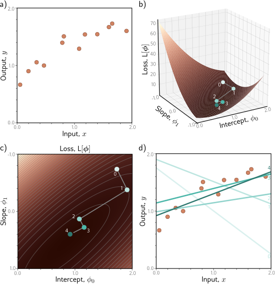
Gradient descent for the linear regression model.

Training set of \(I = 12\) input/output pairs \(\{x_i, y_i\}\).
Loss function showing iterations of gradient descent. We start at point 0 and move in the steepest downhill direction until we can improve no further to arrive at point 1. We then repeat this procedure. We measure the gradient at point 1 and move downhill to point 2 and so on.
This can be visualized better as a heatmap, where the brightness represents the loss. After only four iterations, we are already close to the minimum.
The model with the parameters at point 0 (lightest line) describes the data very badly, but each successive iteration improves the fit. The model with the parameters at point 4 (darkest line) is already a reasonable description of the training data.

Figure above shows the progression of the gradient descent algorithm as we iteratively compute the derivatives according to equations above. In this case, we have used a line search procedure to find the value of \(\alpha\) that decreases the loss the most at each iteration.

Gabor model example

Loss functions for linear regression problems always have a single well-defined global minimum. More formally, they are convex. Convexity implies that wherever we initialize the parameters, we are bound to reach the minimum if we keep walking downhill; the training procedure can’t fail.

Unfortunately, loss functions for most nonlinear models, including both shallow and deep networks, are non-convex. Visualizing neural network loss functions is challenging due to the number of parameters. Hence, we first explore a simpler nonlinear model with two parameters to gain insight into the properties of non-convex loss functions:

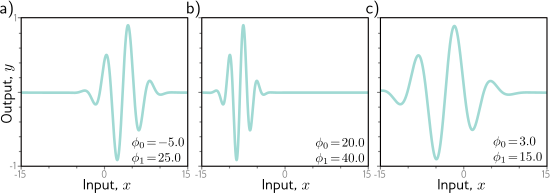
\[\begin{eqnarray}\label{eq:train_gabor} \mbox{f}[x,\boldsymbol\phi] = \sin[\phi_0 + 0.06\cdot\phi_{1}x]\cdot \exp\left(-\frac{(\phi_0+0.06\cdot\phi_{1}x)^2}{32.0}\right). \end{eqnarray}\]

This Gabor model maps scalar input \(x\) to scalar output \(y\) and consists of a sinusoidal component (creating an oscillatory function) multiplied by a negative exponential com- ponent (causing the amplitude to decrease as we move from the center).

It has two parameters \(\phi= [\phi_0,\phi_1]^T\), where \(\phi_0 \in \mathbb{R}\) determines the mean position of the function and \(\phi_1 \in \mathbb{R}^+\) stretches or squeezes it along the x-axis. Consider a training set of \(I\) examples \(\{x_i,y_i\}\)(figure 6.3). The least squares loss function for I training examples is defined as:

\[\begin{eqnarray} L[\boldsymbol\phi] = \sum_{i=1}^{I}\left(\mbox{f}[x_{i},\boldsymbol\phi]-y_{i}\right)^2. \end{eqnarray}\]

Once more, the goal is to find the parameters \(\hat{\phi}\)that minimize this loss.

Gabor model. This nonlinear model maps scalar input \(x\) to scalar output \(y\) and has parameters \(\phi = [\phi_0, \phi_1]^T\). It describes a sinusoidal function that decreases in amplitude with distance from its center. Parameter \(\phi_0 \in \mathbb{R}\) determines the position of the center. As \(\phi_0\) increases, the function moves left. Parameter \(\phi_1 \in \mathbb{R}^+\) squeezes the function along the x-axis relative to the center. As \(ϕ_1\) increases, the function narrows. a–c) Model with different parameters.

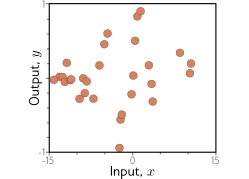
Training data for fitting the Gabor model.

The training dataset contains 28 input/output examples \(\{x_i, y_i\}\).

These data were created by uniformly sampling \(x_i \in [−15, 15]\), passing the samples through a Gabor model with parameters \(\phi = [0.0, 16.6]^T\) , and adding normally distributed noise.

Local minima and saddle points

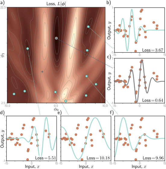
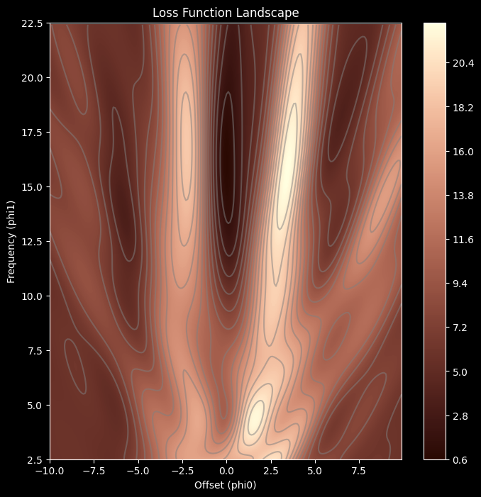
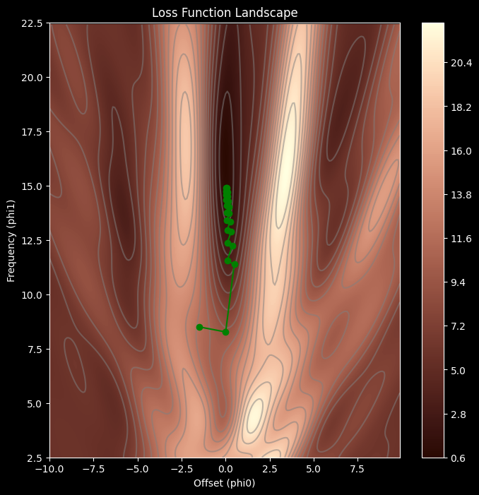
Figure below depicts the loss function associated with the Gabor model for this dataset.

There are numerous local minima (red circles). Here the gradient is zero, and the loss increases if we move in any direction, but we are not at the overall minimum of the function.

The point with the lowest loss is known as the global minimum and is depicted by the gray circle. If we start in a random position and use gradient descent to go downhill, there is no guarantee that we will wind up at the global minimum and find the best parameters. It’s equally or even more likely that the algorithm will terminate in one of the local minima. Furthermore, there is no way of knowing whether there is a better solution elsewhere.

Loss function for the Gabor model. a) The loss function is non-convex, with multiple local minima (cyan circles) in addition to the global minimum (gray circle). It also contains saddle points where the gradient is locally zero, but the function increases in one direction and decreases in the other. The blue cross is an example of a saddle point; the function decreases as we move horizontally in either direction but increases as we move vertically. b–f) Models associated with the different minima. In each case, there is no small change that decreases the loss. Panel (c) shows the global minimum, which has a loss of 0.64. (Interactive figure)

In addition, the loss function contains saddle points (e.g., the beige cross in figure above). At saddle points, the gradient is zero, but the function increases in some directions and decreases in others. If the current parameters are not exactly at the saddle point, then gradient descent can escape by moving downhill. However, the surface near the saddle point is flat, so it’s hard to be sure that training hasn’t converged; if we terminate the algorithm when the gradient is small, we may erroneously stop near a saddle point.

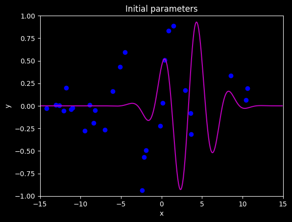
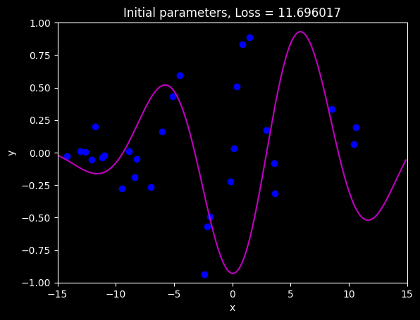
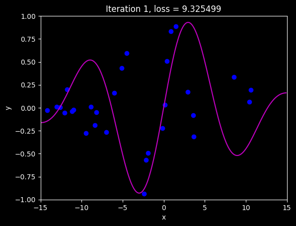
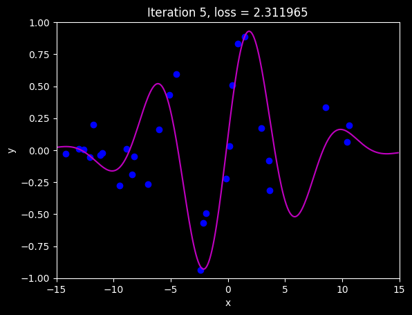
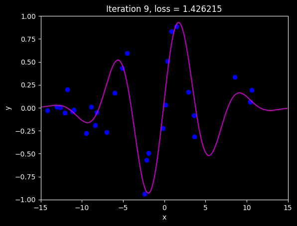
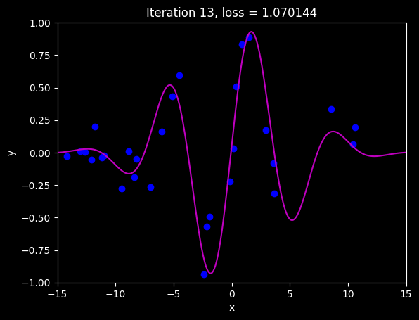
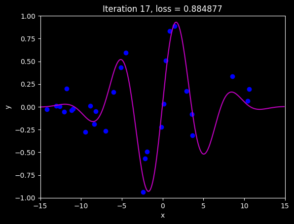
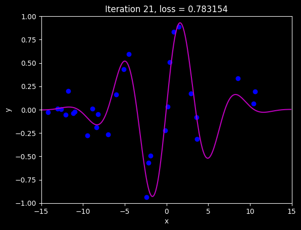
# import libraries
import numpy as np
import matplotlib.pyplot as plt
from matplotlib import cm
from matplotlib.colors import ListedColormap

plt.style.use('dark_background')
     

# Let's create our training data of 30 pairs {x_i, y_i}
# We'll try to fit the Gabor model to these data
data = np.array([[-1.920e+00,-1.422e+01,1.490e+00,-1.940e+00,-2.389e+00,-5.090e+00,
                 -8.861e+00,3.578e+00,-6.010e+00,-6.995e+00,3.634e+00,8.743e-01,
                 -1.096e+01,4.073e-01,-9.467e+00,8.560e+00,1.062e+01,-1.729e-01,
                  1.040e+01,-1.261e+01,1.574e-01,-1.304e+01,-2.156e+00,-1.210e+01,
                 -1.119e+01,2.902e+00,-8.220e+00,-1.179e+01,-8.391e+00,-4.505e+00],
                  [-1.051e+00,-2.482e-02,8.896e-01,-4.943e-01,-9.371e-01,4.306e-01,
                  9.577e-03,-7.944e-02 ,1.624e-01,-2.682e-01,-3.129e-01,8.303e-01,
                  -2.365e-02,5.098e-01,-2.777e-01,3.367e-01,1.927e-01,-2.222e-01,
                  6.352e-02,6.888e-03,3.224e-02,1.091e-02,-5.706e-01,-5.258e-02,
                  -3.666e-02,1.709e-01,-4.805e-02,2.008e-01,-1.904e-01,5.952e-01]])
     

# Let's define our model
def model(phi,x):
  sin_component = np.sin(phi[0] + 0.06 * phi[1] * x)
  gauss_component = np.exp(-(phi[0] + 0.06 * phi[1] * x) * (phi[0] + 0.06 * phi[1] * x) / 32)
  y_pred= sin_component * gauss_component
  return y_pred
     

# Draw model
def draw_model(data,model,phi,title=None):
  x_model = np.arange(-15,15,0.1)
  y_model = model(phi,x_model)

  fix, ax = plt.subplots()
  ax.plot(data[0,:],data[1,:],'bo')
  ax.plot(x_model,y_model,'m-')
  ax.set_xlim([-15,15]);ax.set_ylim([-1,1])
  ax.set_xlabel('x'); ax.set_ylabel('y')
  if title is not None:
    ax.set_title(title)
  plt.show()
     

# Initialize the parameters and draw the model
phi = np.zeros((2,1))
phi[0] =  -5     # Horizontal offset
phi[1] =  25     # Frequency
draw_model(data,model,phi, "Initial parameters")

def compute_loss(data_x, data_y, model, phi):

  y_pred = model(phi,data_x)

  loss = np.sum((y_pred - data_y)**2)

  return loss

loss = compute_loss(data[0,:],data[1,:],model,np.array([[0.6],[-0.2]]))
print('Your loss = %3.3f'%(loss))

Your loss = 16.419, Correct loss = 16.419

def draw_loss_function(compute_loss, data,  model, phi_iters = None):
  # Define pretty colormap
  my_colormap_vals_hex =('2a0902', '2b0a03', '2c0b04', '2d0c05', '2e0c06', '2f0d07', '300d08', '310e09', '320f0a', '330f0b', '34100b', '35110c', '36110d', '37120e', '38120f', '39130f', '3a1410', '3b1411', '3c1511', '3d1612', '3e1613', '3f1713', '401714', '411814', '421915', '431915', '451a16', '461b16', '471b17', '481c17', '491d18', '4a1d18', '4b1e19', '4c1f19', '4d1f1a', '4e201b', '50211b', '51211c', '52221c', '53231d', '54231d', '55241e', '56251e', '57261f', '58261f', '592720', '5b2821', '5c2821', '5d2922', '5e2a22', '5f2b23', '602b23', '612c24', '622d25', '632e25', '652e26', '662f26', '673027', '683027', '693128', '6a3229', '6b3329', '6c342a', '6d342a', '6f352b', '70362c', '71372c', '72372d', '73382e', '74392e', '753a2f', '763a2f', '773b30', '783c31', '7a3d31', '7b3e32', '7c3e33', '7d3f33', '7e4034', '7f4134', '804235', '814236', '824336', '834437', '854538', '864638', '874739', '88473a', '89483a', '8a493b', '8b4a3c', '8c4b3c', '8d4c3d', '8e4c3e', '8f4d3f', '904e3f', '924f40', '935041', '945141', '955242', '965343', '975343', '985444', '995545', '9a5646', '9b5746', '9c5847', '9d5948', '9e5a49', '9f5a49', 'a05b4a', 'a15c4b', 'a35d4b', 'a45e4c', 'a55f4d', 'a6604e', 'a7614e', 'a8624f', 'a96350', 'aa6451', 'ab6552', 'ac6552', 'ad6653', 'ae6754', 'af6855', 'b06955', 'b16a56', 'b26b57', 'b36c58', 'b46d59', 'b56e59', 'b66f5a', 'b7705b', 'b8715c', 'b9725d', 'ba735d', 'bb745e', 'bc755f', 'bd7660', 'be7761', 'bf7862', 'c07962', 'c17a63', 'c27b64', 'c27c65', 'c37d66', 'c47e67', 'c57f68', 'c68068', 'c78169', 'c8826a', 'c9836b', 'ca846c', 'cb856d', 'cc866e', 'cd876f', 'ce886f', 'ce8970', 'cf8a71', 'd08b72', 'd18c73', 'd28d74', 'd38e75', 'd48f76', 'd59077', 'd59178', 'd69279', 'd7937a', 'd8957b', 'd9967b', 'da977c', 'da987d', 'db997e', 'dc9a7f', 'dd9b80', 'de9c81', 'de9d82', 'df9e83', 'e09f84', 'e1a185', 'e2a286', 'e2a387', 'e3a488', 'e4a589', 'e5a68a', 'e5a78b', 'e6a88c', 'e7aa8d', 'e7ab8e', 'e8ac8f', 'e9ad90', 'eaae91', 'eaaf92', 'ebb093', 'ecb295', 'ecb396', 'edb497', 'eeb598', 'eeb699', 'efb79a', 'efb99b', 'f0ba9c', 'f1bb9d', 'f1bc9e', 'f2bd9f', 'f2bfa1', 'f3c0a2', 'f3c1a3', 'f4c2a4', 'f5c3a5', 'f5c5a6', 'f6c6a7', 'f6c7a8', 'f7c8aa', 'f7c9ab', 'f8cbac', 'f8ccad', 'f8cdae', 'f9ceb0', 'f9d0b1', 'fad1b2', 'fad2b3', 'fbd3b4', 'fbd5b6', 'fbd6b7', 'fcd7b8', 'fcd8b9', 'fcdaba', 'fddbbc', 'fddcbd', 'fddebe', 'fddfbf', 'fee0c1', 'fee1c2', 'fee3c3', 'fee4c5', 'ffe5c6', 'ffe7c7', 'ffe8c9', 'ffe9ca', 'ffebcb', 'ffeccd', 'ffedce', 'ffefcf', 'fff0d1', 'fff2d2', 'fff3d3', 'fff4d5', 'fff6d6', 'fff7d8', 'fff8d9', 'fffada', 'fffbdc', 'fffcdd', 'fffedf', 'ffffe0')
  my_colormap_vals_dec = np.array([int(element,base=16) for element in my_colormap_vals_hex])
  r = np.floor(my_colormap_vals_dec/(256*256))
  g = np.floor((my_colormap_vals_dec - r *256 *256)/256)
  b = np.floor(my_colormap_vals_dec - r * 256 *256 - g * 256)
  my_colormap = ListedColormap(np.vstack((r,g,b)).transpose()/255.0)

  # Make grid of offset/frequency values to plot
  offsets_mesh, freqs_mesh = np.meshgrid(np.arange(-10,10.0,0.1), np.arange(2.5,22.5,0.1))
  loss_mesh = np.zeros_like(freqs_mesh)
  # Compute loss for every set of parameters
  for idslope, slope in np.ndenumerate(freqs_mesh):
     loss_mesh[idslope] = compute_loss(data[0,:], data[1,:], model, np.array([[offsets_mesh[idslope]], [slope]]))

  fig,ax = plt.subplots()
  fig.set_size_inches(8,8)
  a = ax.contourf(offsets_mesh,freqs_mesh,loss_mesh,256,cmap=my_colormap)
  ax.contour(offsets_mesh,freqs_mesh,loss_mesh,20,colors=['#80808080'])
  if phi_iters is not None:
    ax.plot(phi_iters[0,:], phi_iters[1,:],'go-')
  ax.set_ylim([2.5,22.5])
  ax.set_xlabel('Offset (phi0)'); ax.set_ylabel('Frequency (phi1)')
  fig.colorbar(a)
  ax.set_title('Loss Function Landscape')
  plt.show()
     

draw_loss_function(compute_loss, data, model)

# These came from writing out the expression for the sum of squares loss and taking the
# derivative with respect to phi0 and phi1. It was a lot of hassle to get it right!
def gabor_deriv_phi0(data_x,data_y,phi0, phi1):
    x = 0.06 * phi1 * data_x + phi0
    y = data_y
    cos_component = np.cos(x)
    sin_component = np.sin(x)
    gauss_component = np.exp(-0.5 * x *x / 16)
    deriv = cos_component * gauss_component - sin_component * gauss_component * x / 16
    deriv = 2* deriv * (sin_component * gauss_component - y)
    return np.sum(deriv)

def gabor_deriv_phi1(data_x, data_y,phi0, phi1):
    x = 0.06 * phi1 * data_x + phi0
    y = data_y
    cos_component = np.cos(x)
    sin_component = np.sin(x)
    gauss_component = np.exp(-0.5 * x *x / 16)
    deriv = 0.06 * data_x * cos_component * gauss_component - 0.06 * data_x*sin_component * gauss_component * x / 16
    deriv = 2*deriv * (sin_component * gauss_component - y)
    return np.sum(deriv)

def compute_gradient(data_x, data_y, phi):
    dl_dphi0 = gabor_deriv_phi0(data_x, data_y, phi[0],phi[1])
    dl_dphi1 = gabor_deriv_phi1(data_x, data_y, phi[0],phi[1])
    # Return the gradient
    return np.array([[dl_dphi0],[dl_dphi1]])

We can check we got this right using a trick known as finite differences. If we evaluate the function and then change one of the parameters by a very small amount and normalize by that amount, we get an approximation to the gradient, so:

We can’t do this when there are many parameters; for a million parameters, we would have to evaluate the loss function two million times, and usually computing the gradients directly is much more efficient.

# Compute the gradient using your function
gradient = compute_gradient(data[0,:],data[1,:], phi)
print("Your gradients: (%3.3f,%3.3f)"%(gradient[0],gradient[1]))
# Approximate the gradients with finite differences
delta = 0.0001
dl_dphi0_est = (compute_loss(data[0,:],data[1,:],model,phi+np.array([[delta],[0]])) - \
                    compute_loss(data[0,:],data[1,:],model,phi))/delta
dl_dphi1_est = (compute_loss(data[0,:],data[1,:],model,phi+np.array([[0],[delta]])) - \
                    compute_loss(data[0,:],data[1,:],model,phi))/delta
print("Approx gradients: (%3.3f,%3.3f)"%(dl_dphi0_est,dl_dphi1_est))

Your gradients: (3.344,0.519)
Approx gradients: (3.344,0.519)

Now we are ready to perform gradient descent. We’ll need to use our line search routine from Notebook 6.1, which I’ve reproduced here plus the helper function loss_function_1D that converts from a 2D problem to a 1D problem

def loss_function_1D(dist_prop, data, model, phi_start, gradient):
  # Return the loss after moving this far
  return compute_loss(data[0,:], data[1,:], model, phi_start+ gradient * dist_prop)

def line_search(data, model, phi, gradient, thresh=.00001, max_dist = 0.1, max_iter = 15, verbose=False):
    # Initialize four points along the range we are going to search
    a = 0
    b = 0.33 * max_dist
    c = 0.66 * max_dist
    d = 1.0 * max_dist
    n_iter = 0

    # While we haven't found the minimum closely enough
    while np.abs(b-c) > thresh and n_iter < max_iter:
        # Increment iteration counter (just to prevent an infinite loop)
        n_iter = n_iter+1
        # Calculate all four points
        lossa = loss_function_1D(a, data, model, phi,gradient)
        lossb = loss_function_1D(b, data, model, phi,gradient)
        lossc = loss_function_1D(c, data, model, phi,gradient)
        lossd = loss_function_1D(d, data, model, phi,gradient)

        if verbose:
          print('Iter %d, a=%3.3f, b=%3.3f, c=%3.3f, d=%3.3f'%(n_iter, a,b,c,d))
          print('a %f, b%f, c%f, d%f'%(lossa,lossb,lossc,lossd))

        # Rule #1 If point A is less than points B, C, and D then change B,C,D so they are half their current distance from A
        if np.argmin((lossa,lossb,lossc,lossd))==0:
          b = a+ (b-a)/2
          c = a+ (c-a)/2
          d = a+ (d-a)/2
          continue;

        # Rule #2 If point b is less than point c then
        #                     point d becomes point c, and
        #                     point b becomes 1/3 between a and new d
        #                     point c becomes 2/3 between a and new d
        if lossb < lossc:
          d = c
          b = a+ (d-a)/3
          c = a+ 2*(d-a)/3
          continue

        # Rule #2 If point c is less than point b then
        #                     point a becomes point b, and
        #                     point b becomes 1/3 between new a and d
        #                     point c becomes 2/3 between new a and d
        a = b
        b = a+ (d-a)/3
        c = a+ 2*(d-a)/3

    # Return average of two middle points
    return (b+c)/2.0
     

def gradient_descent_step(phi, data,  model):
  # Step 1:  Compute the gradient
  gradient = compute_gradient(data[0,:],data[1,:], phi)
  # Step 2:  Update the parameters -- note we want to search in the negative (downhill direction)
  alpha = line_search(data, model, phi, gradient*-1, max_dist = 2.0)
  phi = phi - alpha * gradient
  return phi
     

# Initialize the parameters
n_steps = 21
phi_all = np.zeros((2,n_steps+1))
phi_all[0,0] = -1.5
phi_all[1,0] = 8.5

# Measure loss and draw initial model
loss =  compute_loss(data[0,:], data[1,:], model, phi_all[:,0:1])
draw_model(data,model,phi_all[:,0:1], "Initial parameters, Loss = %f"%(loss))

for c_step in range (n_steps):
  # Do gradient descent step
  phi_all[:,c_step+1:c_step+2] = gradient_descent_step(phi_all[:,c_step:c_step+1],data, model)
  # Measure loss and draw model every 4th step
  if c_step % 4 == 0:
    loss =  compute_loss(data[0,:], data[1,:], model, phi_all[:,c_step+1:c_step+2])
    draw_model(data,model,phi_all[:,c_step+1], "Iteration %d, loss = %f"%(c_step+1,loss))

draw_loss_function(compute_loss, data, model,phi_all)