6.1. Vectors

6.1.1. Scalars

Most everyday mathematics consists of manipulating numbers one at a time. Formally, we call these values scalars.

For example, the temperature in Greenville is a balmy \(72\) degrees Fahrenheit. If you wanted to convert the temperature to Celsius you would evaluate the expression \(c = \frac{5}{9}(f - 32)\), setting \(f = 72\). In this equation, the values \(5\), \(9\), and \(32\) are constant scalars. The variables \(c\) and \(f\) in general represent unknown scalars.

We denote scalars by ordinary lower-cased letters (e.g. \(x\), \(y\), and \(z\)) and the space of all (continuous) real-valued scalars by \(\mathbb{R}\). The expression \(x \in \mathbb{R}\) is a formal way to say that \(x\) is a real-valued scalar. The symbol \(\in\) (pronounced “in”) denotes membership in a set. For example, \(x, y \in {0, 1}\) indicates that \(x\) and \(y\) are variables that can only take on values of \(0\) or \(1\).

Scalars in Python are represented by numeric types such as int and float.

x = 3
y = 2

print("x+y:", x+y, "x-y:", x-y, "x*y:", x*y, "x/y:", x/y, "x**y:", x**y)

6.1.2. Vectors

For current purposes, you can think of a vector as a fixed-length array of scalars. As with their code counterparts, we call these scalars the elements of the vector (synonyms include entries and components).

We denote vectors by bold lowercase letters, (e.g., \(\mathbf{x}\), \(\mathbf{y}\), and \(\mathbf{z}\)). The vector of all ones is denoted \(\mathbf{1}\). The vector of all zeros is denoted \(\mathbf{0}\).

The unit vector \(e_i\) is a vector of all 0’s, except entry \(i\), which has value 1:

\[ e_i = (0, \ldots 0, 1, 0, \ldots 0) \]

This is also called a one-hot vector.

We can refer to an element of a vector by using a subscript. For example, \(x_2\) denotes the second element of \(\mathbf{x}\). Since \(x_2\) is a scalar, we do not bold it. By default, we visualize vectors by stacking their elements vertically.

0-based indexing vs. 1-based indexing

In Python, as in most programming languages, vector indices start at \(0\). This is known as zero-based indexing.

In linear algebra, however, subscripts begin at \(1\) (one-based indexing).

A vector \(\mathbf{x} ∈ \mathbb{R}^n\) is a list of \(n\) numbers, usually written as a column vector

\[\begin{split} \mathbf{x} = \begin{bmatrix} x_1 \\ x_2 \\ \vdots \\ x_n \end{bmatrix} \end{split}\]

Here \(x_1 \ldots x_n \) are elements of the vector. Later on, we will distinguish between such column vectors and row vectors whose elements are stacked horizontally.

Vectors are implemented in Python as list or tuples. In pandas, we have for vectors pd.Series which additionally has labels for each value. In general, such pd.Series can have arbitrary lengths, subject to memory limitations.

import pandas as pd 
x = pd.Series(range(10, 100, 10))

x

0    10
1    20
2    30
3    40
4    50
5    60
6    70
7    80
8    90
dtype: int64

Fundamentally, a vector is a list of numbers such as the Python list below.

v = [1, 7, 0, 1]

Mathematicians most often write this as either a column or row vector, which is to say either as

\[\begin{split}\mathbf{x} = \begin{bmatrix}1\\7\\0\\1\end{bmatrix}\end{split}\]

or

\[\mathbf{x}^\top = \begin{bmatrix}1 & 7 & 0 & 1\end{bmatrix}.\]

6.1.2.1. Geometry of Vectors

First, we need to discuss the two common geometric interpretations of vectors, as either points or directions in space.

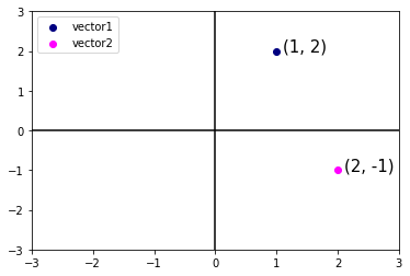
Given a vector, the first interpretation that we should give it is as a point in space. In two or three dimensions, we can visualize these points by using the components of the vectors to define the location of the points in space compared to a fixed reference called the origin. This can be seen in the figure below.

Fig. 6.1 An illustration of visualizing vectors as points in the plane. The first component of the vector gives the \(x\)-coordinate, the second component gives the \(y\)-coordinate. Higher dimensions are analogous, although much harder to visualize.

This geometric point of view allows us to consider the problem on a more abstract level. No longer faced with some insurmountable seeming problem like classifying pictures as either cats or dogs, we can start considering tasks abstractly as collections of points in space and picturing the task as discovering how to separate two distinct clusters of points.

import pandas as pd 
from matplotlib import pyplot as plt

plt.xlim(-3, 3)
plt.ylim(-3, 3)

vector1 = [1, 2]
vector2 = [2, -1]

displacement = 0.1

# Plotting vector 1
plt.scatter(x=vector1[0], y=vector1[1], color='navy');
plt.text(x=vector1[0]+displacement, y=vector1[1], \
             s=f"(%s, %s)" % (vector1[0], vector1[1]), size=15);

# Plotting vector 2
plt.scatter(x=vector2[0], y=vector2[1], color='magenta');
plt.text(x=vector2[0]+displacement, y=vector2[1], \
             s=f"(%s, %s)" % (vector2[0], vector2[1]), size=15);

# Plotting the x and y axes
plt.axhline(0, color='black');
plt.axvline(0, color='black');

# Plotting the legend
plt.legend(['vector1', 'vector2'], loc='upper left');

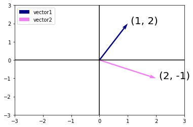
In parallel, there is a second point of view that people often take of vectors: as directions in space. Not only can we think of the vector \(\textbf{v} = [3, 2]^{T}\) as the location \(3\) units to the right and \(2\) units up from the origin, we can also think of it as the direction itself to take \(3\) steps to the right and \(2\) steps up. In this way, we consider all the vectors in figure below the same.

Fig. 6.2 Any vector can be visualized as an arrow in the plane. In this case, every vector drawn is a representation of the vector \((3, 2)^\top\)

plt.xlim(-3, 3)
plt.ylim(-3, 3)

# Plotting vector 1
plt.quiver(0, 0, vector1[0], vector1[1], scale=1, scale_units='xy', angles='xy', color='navy')
plt.text(x=vector1[0]+displacement, y=vector1[1], \
             s=f"(%s, %s)" % (vector1[0], vector1[1]), size=20);

# Plotting vector 2
plt.quiver(0, 0, vector2[0], vector2[1], scale=1, scale_units='xy', angles='xy', color='violet')
plt.text(x=vector2[0]+displacement, y=vector2[1], \
             s=f"(%s, %s)" % (vector2[0], vector2[1]), size=20);

plt.legend(['vector1', 'vector2'], loc='upper left');

# Plotting the x and y axes
plt.axhline(0, color='black');
plt.axvline(0, color='black');

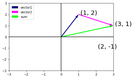
One of the benefits of this shift is that we can make visual sense of the act of vector addition. In particular, we follow the directions given by one vector, and then follow the directions given by the other, as seen below:

Fig. 6.3 We can visualize vector addition by first following one vector, and then another.

Vector subtraction has a similar interpretation. By considering the identity that \(\mathbf{u} = \mathbf{v} + (\mathbf{u} - \mathbf{v})\), we see that the vector \(\mathbf{u} - \mathbf{v}\) is the direction that takes us from the point \(\mathbf{v}\) to the point \(\mathbf{u}\).

vector1 = df[['x', 'y']].iloc[0]
vector2 = df[['x', 'y']].iloc[1]

sum = vector1 + vector2

sum = pd.Series(vector1) + pd.Series(vector2)

sum

0    4
1    6
dtype: int64

vector1 = pd.Series([1, 2])
vector2 = pd.Series([2, -1])
sum = vector1 + vector2

plt.xlim(-3, 3)
plt.ylim(-3, 3)

# Plotting vector 1
plt.quiver(0, 0, vector1[0], vector1[1], scale=1, scale_units='xy', angles='xy', color='navy')
plt.text(x=vector1[0]+displacement, y=vector1[1], \
             s=f"(%s, %s)" % (vector1[0], vector1[1]), size=20);

# Plotting vector 2
plt.quiver(vector1[0], vector1[1], vector2[0], vector2[1], scale=1, scale_units='xy', angles='xy', color='magenta')
plt.text(x=vector2[0]+displacement, y=vector2[1], \
             s=f"(%s, %s)" % (vector2[0], vector2[1]), size=20);


plt.quiver(0, 0, sum[0], sum[1], scale=1, scale_units='xy', angles='xy', color='lime')
plt.text(x=sum[0]+displacement, y=sum[1], \
             s=f"(%s, %s)" % (sum[0], sum[1]), size=20);

plt.legend(['vector1', 'vector2', 'sum'], loc='upper left');

# Plotting the x and y axes
plt.axhline(0, color='black');
plt.axvline(0, color='black');

6.1.2.2. Norms

Some of the most useful operators in linear algebra are norms. A norm is a function \(\| \cdot \|\) that maps a vector to a scalar.

Informally, the norm of a vector tells us magnitude or length of the vector.

For instance, the \(l_2\) norm measures the euclidean length of a vector. That is, \(l_2\) norm measures the euclidean distance of a vector from the origin \((0, 0)\).

\[ \|\mathbf{x}\|_2 = \sqrt{\sum_{i=1}^n x_i^2} \]

x = pd.Series(vector1)
l2_norm = (x**2).sum()**(1/2)
l2_norm

2.23606797749979

The \(l_1\) norm is also common and the associated measure is called the Manhattan distance. By definition, the \(l_1\) norm sums the absolute values of a vector’s elements:

\[ \|\mathbf{x}\|_1 = \sum_{i=1}^n \left|x_i \right| \]

Compared to the \(l_2\) norm, it is less sensitive to outliers. To compute the \(l_1\) norm, we compose the absolute value with the sum operation.

l1_norm = x.abs().sum()
l1_norm

6

Both the \(l_1\) and \(l_2\) norms are special cases of the more general norms:

\[ \|\mathbf{x}\|_p = \left(\sum_{i=1}^n \left|x_i \right|^p \right)^{1/p}. \]

vec = pd.Series([1, 2, 3, 4, 5, 6, 7, 8, 9])

p = 3

lp_norm = ((abs(vec))**p).sum()**(1/p)

lp_norm

12.651489979526238

6.1.2.3. Dot Product

One of the most fundamental operations in linear algebra (and all of data science and machine learning) is the dot product.

Given two vectors \(\textbf{x}, \textbf{y} \in \mathbb{R}^d\), their dot product \(\textbf{x}^{\top} \textbf{y}\) (also known as inner product \(\langle \textbf{x}, \textbf{y} \rangle\)) is a sum over the products of the elements at the same position:

\[\textbf{x}^\top \textbf{y} = \sum_{i=1}^{d} x_i y_i\]

import pandas as pd

x = pd.Series([1, 2, 3])
y = pd.Series([4, 5, 6])

x.dot(y) # 1*4 + 2*5 + 3*6 

32

Equivalently, we can calculate the dot product of two vectors by performing an elementwise multiplication followed by a sum:

sum(x * y)

32

Dot products are useful in a wide range of contexts. For example, given some set of values, denoted by a vector \( \mathbf{x} \in \mathbb{R}^{n} \) , and a set of weights, denoted by \(\mathbf{x} \in \mathbb{R}^{n}\), the weighted sum of the values in \(\mathbf{x}\) according to the weights \(\mathbf{w}\) could be expressed as the dot product \(\mathbf{x}^\top \mathbf{w}\). When the weights are nonnegative and sum to \(1\), i.e., \((\sum_{i=1}^n w_i = 1)\), the dot product expresses a weighted average. After normalizing two vectors to have unit length, the dot products express the cosine of the angle between them. Later in this section, we will formally introduce this notion of length.

6.1.2.4. Dot Products and Angles

If we take two column vectors \(\mathbf{u}\) and \(\mathbf{v}\), we can form their dot product by computing:

\[ \mathbf{u}^\top\mathbf{v} = \sum_i u_i\cdot v_i \]

Because the equation above is symmetric, we will mirror the notation of classical multiplication and write

\[ \mathbf{u}\cdot\mathbf{v} = \mathbf{u}^\top\mathbf{v} = \mathbf{v}^\top\mathbf{u}, \]

to highlight the fact that exchanging the order of the vectors will yield the same answer.

The dot product also admits a geometric interpretation: dot product it is closely related to the angle between two vectors.

Fig. 6.4 Between any two vectors in the plane there is a well defined angle \(\theta\). We will see this angle is intimately tied to the dot product.

To start, let’s consider two specific vectors:

\[ \mathbf{v} = (r,0) \; \textrm{and} \; \mathbf{w} = (s\cos(\theta), s \sin(\theta)) \]

The vector \(\mathbf{v}\) is length \(r\) and runs parallel to the \(x\)-axis, and the vector \(\mathbf{w}\) is of length \(s\) and at angle \(\theta\) with the \(x\)-axis.

If we compute the dot product of these two vectors, we see that

\[ \mathbf{v}\cdot\mathbf{w} = rs\cos(\theta) = \|\mathbf{v}\|\|\mathbf{w}\|\cos(\theta) \]

With some simple algebraic manipulation, we can rearrange terms to obtain the equation for any two vectors \(\mathbf{v}\) and \(\mathbf{w}\):

\[ \theta = \arccos\left(\frac{\mathbf{v}\cdot\mathbf{w}}{\|\mathbf{v}\|\|\mathbf{w}\|}\right) \]

We will not use it right now, but it is useful to know that we will refer to vectors for which the angle is \(\pi/2\)(or equivalently \(90^{\circ}\)) as being orthogonal.

By examining the equation above, we see that this happens when \(\theta = \pi/2\), which is the same thing as \(cos(\theta) = 0\).

The only way this can happen is if the dot product itself is zero, and two vectors are orthogonal if and only if \(\mathbf{v}\cdot\mathbf{w} = 0\).

This will prove to be a helpful formula when understanding objects geometrically.

It is reasonable to ask: why is computing the angle useful? Consider the problem of classifying text data. We might want the topic or sentiment in the text to not change if we write twice as long of document that says the same thing.

For some encoding (such as counting the number of occurrences of words in some vocabulary), this corresponds to a doubling of the vector encoding the document, so again we can use the angle.

v = pd.Series([0, 2])
w = pd.Series([2, 0])

v.dot(w)

0

from math import acos

def l2_norm(vec):
    return (vec**2).sum()**(1/2)

v = pd.Series([0, 2])
w = pd.Series([2, 0])

v.dot(w) / (l2_norm(v) * l2_norm(w))

0.0

from math import acos, pi

theta = acos(v.dot(w) / (l2_norm(v) * l2_norm(w)))

theta == pi / 2

True

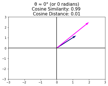
6.1.2.5. Cosine Similarity/Distance

In ML contexts where the angle is employed to measure the closeness of two vectors, practitioners adopt the term cosine similarity to refer to the portion

\[ \cos(\theta) = \frac{\mathbf{v}\cdot\mathbf{w}}{\|\mathbf{v}\|\|\mathbf{w}\|}. \]

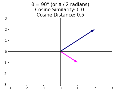
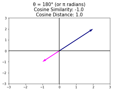
The cosine takes a maximum value of \(1\) when the two vectors point in the same direction, a minimum value of \(-1\) when they point in opposite directions, and a value of \(0\) when the two vectors are orthogonal.

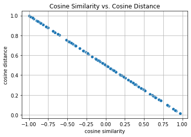
Note that cosine similarity can be converted to cosine distance by subtracting it from \(1\) and dividing by 2.

\[ \text{Cosine Distance} = \frac{1 - \text{Cosine Similarity}}{2}\]

where \(\text{Cosine Similarity} = \frac{\mathbf{v}\cdot\mathbf{w}}{\|\mathbf{v}\|\|\mathbf{w}\|}\)

Cosine distance is a very useful alternative to Euclidean distance for data where the absolute magnitude of the features is not particularly meaningful, which is a very common scenario in practice.

from random import uniform
import pandas as pd
import seaborn as sns

df = pd.DataFrame()
df['cosine similarity'] = pd.Series([uniform(-1, 1) for i in range(100)])
df['cosine distance']   = (1 - df['cosine similarity'])/2
ax = sns.scatterplot(data=df, x='cosine similarity', y='cosine distance');
ax.set(title='Cosine Similarity vs. Cosine Distance')
plt.grid()

def l2_norm(vec):
    return (vec**2).sum()**(1/2)

plt.axhline(0, color='black');
plt.axvline(0, color='black');

v = pd.Series([1.2, 1.2])
w = pd.Series([2, 2.5])

plt.quiver(0, 0, v[0], v[1], scale=1, scale_units='xy', angles='xy', color='navy')
plt.quiver(0, 0, w[0], w[1], scale=1, scale_units='xy', angles='xy', color='magenta')

plt.xlim(-3, 3)
plt.ylim(-3, 3)

cosine_similarity = v.dot(w) / (l2_norm(v) * l2_norm(w))
cosine_similarity = round(cosine_similarity, 2)

cosine_distance = (1 - cosine_similarity) / 2
cosine_distance = round(cosine_distance, 2)

plt.title("θ ≈ 0° (or 0 radians)\n"+\
          "Cosine Similarity: %s \nCosine Distance: %s" % \
          (cosine_similarity, cosine_distance), size=15);

plt.axhline(0, color='black');
plt.axvline(0, color='black');

v = pd.Series([2, 2])
w = pd.Series([1, -1])

plt.quiver(0, 0, v[0], v[1], scale=1, scale_units='xy', angles='xy', color='navy')
plt.quiver(0, 0, w[0], w[1], scale=1, scale_units='xy', angles='xy', color='magenta')

plt.xlim(-3, 3)
plt.ylim(-3, 3)

cosine_similarity = v.dot(w) / (l2_norm(v) * l2_norm(w))
cosine_similarity = round(cosine_similarity, 2)


cosine_distance = (1 - cosine_similarity) / 2
cosine_distance = round(cosine_distance, 2)

plt.title("θ = 90° (or π / 2 radians)"+\
          "\nCosine Similarity: %s "+\
          "\nCosine Distance: %s" % \
          (cosine_similarity, cosine_distance), size=15);

Note that cosine similarity can be negative, which means that the angle is greater than \(90^{\circ}\), i.e., the vectors point in opposite directions.

v = pd.Series([2, 2])
w = pd.Series([-1, -1])

plt.quiver(0, 0, v[0], v[1], scale=1, scale_units='xy', angles='xy', color='navy')
plt.quiver(0, 0, w[0], w[1], scale=1, scale_units='xy', angles='xy', color='magenta')

plt.xlim(-3, 3)
plt.ylim(-3, 3)

plt.axhline(0, color='black');
plt.axvline(0, color='black');

cosine_similarity = v.dot(w) / (l2_norm(v) * l2_norm(w))

cosine_similarity = round(cosine_similarity, 2)

cosine_distance = (1 - cosine_similarity) / 2
cosine_distance = round(cosine_distance, 2)

plt.title("θ = 180° (or π radians)\n"+\
          "Cosine Similarity: %s \nCosine Distance: %s" % \
          (cosine_similarity, cosine_distance), size=15);

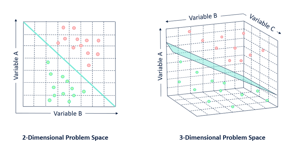
6.1.3. Hyperplanes

In addition to working with vectors, another key object that you must understand to go far in linear algebra is the hyperplane, a generalization to higher dimensions of a line (two dimensions) or of a plane (three dimensions). In an -dimensional vector space, a hyperplane has dimensions and divides the space into two half-spaces.

Let’s start with an example. Suppose that we have a column vector \(\mathbf{w}=[2,1]^\top\). We want to know, “what are the points \(\mathbf{v}\) with \(\mathbf{w}\cdot\mathbf{v} = 1\)?” We can define \(\mathbf{v} = [x, y]\)

\[ \mathbf{w}\cdot\mathbf{v} = 1\]

\[ [2, 1]^\top \cdot [x, y] = 1\]

\[ 2x + y = 1\]

\[ y = -2x + 1\]

Recall that the equation for a line is \(y = mx + b\). Therefore, in the equations above, we have defined a line where the slope (\(m\)) is \(-2\) and the intercept (\(b\)) is \(1\).

In this way, we have found a way to cut our space into two halves, where all the points on one side have dot product below a threshold, and the other side above as we see below:

Fig. 6.5 If we now consider the inequality version of the expression, we see that our hyperplane (in this case: just a line) separates the space into two halves.

The story in higher dimension is much the same. If we now take \(\mathbf{w} = [1,2,3]^\top\) and ask about the points in three dimensions with \(\mathbf{w}\cdot\mathbf{v} = 1\), we obtain a plane at right angles to the given vector \(\mathbf{w}\). The two inequalities again define the two sides of the plane as is shown below:

Fig. 6.6 Hyperplanes in any dimension separate the space into two halves.

While our ability to visualize runs out at this point, nothing stops us from doing this in tens, hundreds, or billions of dimensions. This occurs often when thinking about machine learned models.

For instance, we can understand linear classification models, as methods to find hyperplanes that separate the different target classes. In this context, such hyperplanes are often referred to as decision planes. The majority of deep learned classification models end with a linear layer fed into a softmax, so one can interpret the role of the deep neural network to be to find a non-linear embedding such that the target classes can be separated cleanly by hyperplanes.