1.4. Pandas IV: Aggregation

In this notebook, we will learn how to aggregate data using pandas. This generally entails grouping data by a certain column’s values and then applying a function to the groups.

1.4.1. Aggregation with .groupby

Up until this point, we have been working with individual rows of DataFrames. As data scientists, we often wish to investigate trends across a larger subset of our data. For example, we may want to compute some summary statistic (the mean, median, sum, etc.) for a group of rows in our DataFrame. To do this, we’ll use pandas GroupBy objects.

Fig. 1.26 GroupBy operation broken down into split-apply-combine steps.

Fig. 1.27 Value counts for a single column.

Fig. 1.28 Detail of the split-apply-combine operation.

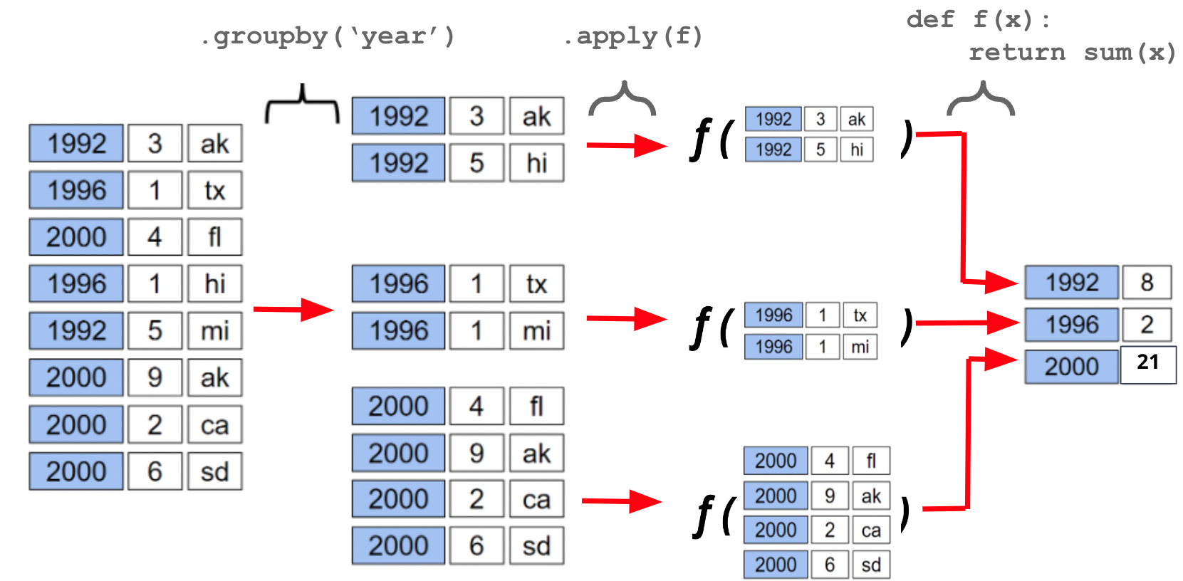
A groupby operation involves some combination of splitting a DataFrame into grouped subframes, applying a function, and combining the results.

For some arbitrary DataFrame df below, the code df.groupby("year").sum() does the following:

• Splits the DataFrame into sub-DataFrames with rows belonging to the same year.

• Applies the sum function to each column of each sub-DataFrame.

• Combines the results of sum into a single DataFrame, indexed by year.

Let’s say we had baby names for all years in a single DataFrame names

Show code cell source Hide code cell source

import urllib.request
import os.path
import pandas as pd 

# Download data from the web directly
data_url = "https://www.ssa.gov/oact/babynames/names.zip"
local_filename = "../data/names.zip"
if not os.path.exists(local_filename): # if the data exists don't download again
    with urllib.request.urlopen(data_url) as resp, open(local_filename, 'wb') as f:
        f.write(resp.read())

        
# Load data without unzipping the file
import zipfile
names = [] 
with zipfile.ZipFile(local_filename, "r") as zf:
    data_files = [f for f in zf.filelist if f.filename[-3:] == "txt"]
    def extract_year_from_filename(fn):
        return int(fn[3:7])
    for f in data_files:
        year = extract_year_from_filename(f.filename)
        with zf.open(f) as fp:
            df = pd.read_csv(fp, names=["Name", "Sex", "Count"])
            df["Year"] = year
            names.append(df)
names = pd.concat(names)

names

	Name	Sex	Count	Year
0	Mary	F	7065	1880
1	Anna	F	2604	1880
2	Emma	F	2003	1880
3	Elizabeth	F	1939	1880
4	Minnie	F	1746	1880
...	...	...	...	...
31677	Zyell	M	5	2023
31678	Zyen	M	5	2023
31679	Zymirr	M	5	2023
31680	Zyquan	M	5	2023
31681	Zyrin	M	5	2023

2117219 rows × 4 columns

names.to_csv("../data/names.csv", index=False)

Now, if we wanted to aggregate all rows in names for a given year, we would need names.groupby("Year")

names.groupby("Year")

<pandas.core.groupby.generic.DataFrameGroupBy object at 0x7f7a30b64bb0>

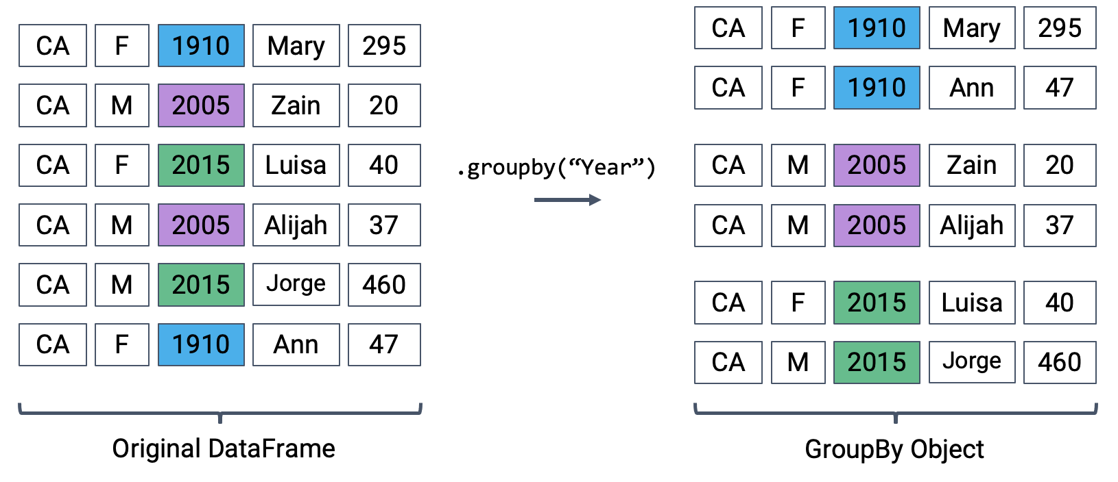
What does this strange output mean? Calling .groupby has generated a GroupBy object. You can imagine this as a set of “mini” sub-DataFrames, where each subframe contains all of the rows from names that correspond to a particular year.

The diagram below shows a simplified view of names to help illustrate this idea.

We can’t work with a GroupBy object directly – that is why you saw that strange output earlier, rather than a standard view of a DataFrame. To actually manipulate values within these “mini” DataFrames, we’ll need to call an aggregation method. This is a method that tells pandas how to aggregate the values within the GroupBy object. Once the aggregation is applied, pandas will return a normal (now grouped) DataFrame.

Aggregation functions (.min(), .max(), .mean(), .sum(), etc.) are the most common way to work with GroupBy objects. These functions are applied to each column of a “mini” grouped DataFrame. We end up with a new DataFrame with one aggregated row per subframe. Let’s see this in action by finding the sum of all counts for each year in names – this is equivalent to finding the number of babies born in each year.

names.groupby("Year").sum().head(5)

	Count
Year
1880	201484
1881	192690
1882	221533
1883	216944
1884	243461

We can relate this back to the diagram we used above. Remember that the diagram uses a simplified version of names, which is why we see smaller values for the summed counts.

Calling .agg has condensed each subframe back into a single row. This gives us our final output: a DataFrame that is now indexed by "Year", with a single row for each unique year in the original names DataFrame.

You may be wondering: where did the "State", "Sex", and "Name" columns go? Logically, it doesn’t make sense to sum the string data in these columns (how would we add “Mary” + “Ann”?). Because of this, pandas will simply omit these columns when it performs the aggregation on the DataFrame. Since this happens implicitly, without the user specifying that these columns should be ignored, it’s easy to run into troubling situations where columns are removed without the programmer noticing. It is better coding practice to select only the columns we care about before performing the aggregation.

# Same result, but now we explicitly tell pandas to only consider the "Count" column when summing
names.groupby("Year")[["Count"]].sum().head(5)

	Count
Year
1880	201484
1881	192690
1882	221533
1883	216944
1884	243461

There are many different aggregations that can be applied to the grouped data. The primary requirement is that an aggregation function must:

• Take in a Series of data (a single column of the grouped subframe)

• Return a single value that aggregates this Series

Because of this fairly broad requirement, pandas offers many ways of computing an aggregation.

In-built Python operations – such as sum, max, and min – are automatically recognized by pandas.

# What is the maximum count for each name in any year?
names.groupby("Name")[["Count"]].max().head()

	Count
Name
Aaban	16
Aabha	9
Aabid	6
Aabidah	5
Aabir	5

# What is the minimum count for each name in any year?
names.groupby("Name")[["Count"]].min().head()

	Count
Name
Aaban	5
Aabha	5
Aabid	5
Aabidah	5
Aabir	5

# What is the average count for each name across all years?
names.groupby("Name")[["Count"]].mean().head()

	Count
Name
Aaban	10.000000
Aabha	6.375000
Aabid	5.333333
Aabidah	5.000000
Aabir	5.000000

pandas also offers a number of in-built functions for aggregation. Some examples include:

• .sum()

• .max()

• .min()

• .mean()

• .first()

• .last()

The latter two entries in this list – "first" and "last" – are unique to pandas. They return the first or last entry in a subframe column. Why might this be useful? Consider a case where multiple columns in a group share identical information. To represent this information in the grouped output, we can simply grab the first or last entry, which we know will be identical to all other entries.

Let’s illustrate this with an example. Say we add a new column to names that contains the first letter of each name.

# Imagine we had an additional column, "First Letter". We'll explain this code next week
names["First Letter"] = names["Name"].apply(lambda x: x[0])

# We construct a simplified DataFrame containing just a subset of columns
names_new = names[["Name", "First Letter", "Year"]]
names_new.head()

	Name	First Letter	Year
0	Mary	M	1880
1	Anna	A	1880
2	Emma	E	1880
3	Elizabeth	E	1880
4	Minnie	M	1880

If we form groups for each name in the dataset, "First Letter" will be the same for all members of the group. This means that if we simply select the first entry for "First Letter" in the group, we’ll represent all data in that group.

We can use a dictionary to apply different aggregation functions to each column during grouping.

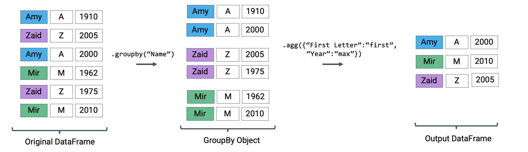
names_new.groupby("Name").agg({"First Letter":"first", "Year":"max"}).head()

	First Letter	Year
Name
Aaban	A	2019
Aabha	A	2021
Aabid	A	2018
Aabidah	A	2018
Aabir	A	2018

We can also define aggregation functions of our own! This can be done using either a def or lambda statement. Again, the condition for a custom aggregation function is that it must take in a Series and output a single scalar value.

def ratio_to_peak(series):
    return series.iloc[-1]/max(series)

names.groupby("Name")[["Year", "Count"]].apply(ratio_to_peak)

---------------------------------------------------------------------------
NameError                                 Traceback (most recent call last)
Input In [2], in <cell line: 4>()
      1 def ratio_to_peak(series):
      2     return series.iloc[-1]/max(series)
----> 4 names.groupby("Name")[["Year", "Count"]].apply(ratio_to_peak)

NameError: name 'names' is not defined

Note

lambda functions are a special type of function that can be defined in a single line. They are also often refered to as “anonymous” functions because these functions don’t have a name. They are useful for simple functions that are not used elsewhere in your code.

# Alternatively, using lambda
names.groupby("Name")[["Year", "Count"]].agg(lambda s: s.iloc[-1]/max(s))

	Year	Count
Name
Aaban	1.0	0.375000
Aabha	1.0	0.555556
Aabid	1.0	1.000000
Aabidah	1.0	1.000000
Aabir	1.0	1.000000
...	...	...
Zyvion	1.0	1.000000
Zyvon	1.0	1.000000
Zyyanna	1.0	1.000000
Zyyon	1.0	1.000000
Zzyzx	1.0	1.000000

101338 rows × 2 columns

1.4.1.1. Aggregation with lambda Functions

We’ll work with the elections DataFrame again.

import pandas as pd

url = "https://raw.githubusercontent.com/fahadsultan/csc272/main/data/elections.csv"
elections = pd.read_csv(url)
elections.head(5)

	Year	Candidate	Party	Popular vote	Result	%
0	1824	Andrew Jackson	Democratic-Republican	151271	loss	57.210122
1	1824	John Quincy Adams	Democratic-Republican	113142	win	42.789878
2	1828	Andrew Jackson	Democratic	642806	win	56.203927
3	1828	John Quincy Adams	National Republican	500897	loss	43.796073
4	1832	Andrew Jackson	Democratic	702735	win	54.574789

What if we wish to aggregate our DataFrame using a non-standard function – for example, a function of our own design? We can do so by combining .agg with lambda expressions.

Let’s first consider a puzzle to jog our memory. We will attempt to find the Candidate from each Party with the highest % of votes.

A naive approach may be to group by the Party column and aggregate by the maximum.

elections.groupby("Party").agg(max).head(10)

	Year	Candidate	Popular vote	Result	%
Party
American	1976	Thomas J. Anderson	873053	loss	21.554001
American Independent	1976	Lester Maddox	9901118	loss	13.571218
Anti-Masonic	1832	William Wirt	100715	loss	7.821583
Anti-Monopoly	1884	Benjamin Butler	134294	loss	1.335838
Citizens	1980	Barry Commoner	233052	loss	0.270182
Communist	1932	William Z. Foster	103307	loss	0.261069
Constitution	2016	Michael Peroutka	203091	loss	0.152398
Constitutional Union	1860	John Bell	590901	loss	12.639283
Democratic	2020	Woodrow Wilson	81268924	win	61.344703
Democratic-Republican	1824	John Quincy Adams	151271	win	57.210122

This approach is clearly wrong – the DataFrame claims that Woodrow Wilson won the presidency in 2020.

Why is this happening? Here, the max aggregation function is taken over every column independently. Among Democrats, max is computing:

• The most recent Year a Democratic candidate ran for president (2020)

• The Candidate with the alphabetically “largest” name (“Woodrow Wilson”)

• The Result with the alphabetically “largest” outcome (“win”)

Instead, let’s try a different approach. We will:

1. Sort the DataFrame so that rows are in descending order of %

2. Group by Party and select the first row of each sub-DataFrame

While it may seem unintuitive, sorting elections by descending order of % is extremely helpful. If we then group by Party, the first row of each groupby object will contain information about the Candidate with the highest voter %.

elections_sorted_by_percent = elections.sort_values("%", ascending=False)
elections_sorted_by_percent.head(5)

	Year	Candidate	Party	Popular vote	Result	%
114	1964	Lyndon Johnson	Democratic	43127041	win	61.344703
91	1936	Franklin Roosevelt	Democratic	27752648	win	60.978107
120	1972	Richard Nixon	Republican	47168710	win	60.907806
79	1920	Warren Harding	Republican	16144093	win	60.574501
133	1984	Ronald Reagan	Republican	54455472	win	59.023326

elections_sorted_by_percent.groupby("Party").agg(lambda x : x.iloc[0]).head(10)

# Equivalent to the below code
# elections_sorted_by_percent.groupby("Party").agg('first').head(10)

	Year	Candidate	Popular vote	Result	%
Party
American	1856	Millard Fillmore	873053	loss	21.554001
American Independent	1968	George Wallace	9901118	loss	13.571218
Anti-Masonic	1832	William Wirt	100715	loss	7.821583
Anti-Monopoly	1884	Benjamin Butler	134294	loss	1.335838
Citizens	1980	Barry Commoner	233052	loss	0.270182
Communist	1932	William Z. Foster	103307	loss	0.261069
Constitution	2008	Chuck Baldwin	199750	loss	0.152398
Constitutional Union	1860	John Bell	590901	loss	12.639283
Democratic	1964	Lyndon Johnson	43127041	win	61.344703
Democratic-Republican	1824	Andrew Jackson	151271	loss	57.210122

Here’s an illustration of the process:

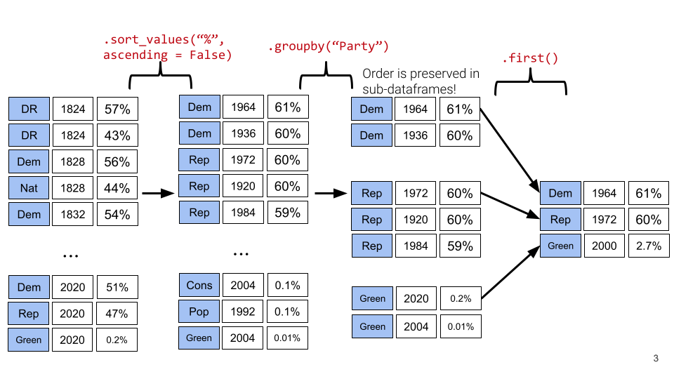
Notice how our code correctly determines that Lyndon Johnson from the Democratic Party has the highest voter %.

More generally, lambda functions are used to design custom aggregation functions that aren’t pre-defined by Python. The input parameter x to the lambda function is a GroupBy object. Therefore, it should make sense why lambda x : x.iloc[0] selects the first row in each groupby object.

In fact, there’s a few different ways to approach this problem. Each approach has different tradeoffs in terms of readability, performance, memory consumption, complexity, etc. We’ve given a few examples below.

Note: Understanding these alternative solutions is not required. They are given to demonstrate the vast number of problem-solving approaches in pandas.

# Using the idxmax function
best_per_party = elections.loc[elections.groupby('Party')['%'].idxmax()]
best_per_party.head(5)

	Year	Candidate	Party	Popular vote	Result	%
22	1856	Millard Fillmore	American	873053	loss	21.554001
115	1968	George Wallace	American Independent	9901118	loss	13.571218
6	1832	William Wirt	Anti-Masonic	100715	loss	7.821583
38	1884	Benjamin Butler	Anti-Monopoly	134294	loss	1.335838
127	1980	Barry Commoner	Citizens	233052	loss	0.270182

# Using the .drop_duplicates function
best_per_party2 = elections.sort_values('%').drop_duplicates(['Party'], keep='last')
best_per_party2.head(5)

	Year	Candidate	Party	Popular vote	Result	%
148	1996	John Hagelin	Natural Law	113670	loss	0.118219
164	2008	Chuck Baldwin	Constitution	199750	loss	0.152398
110	1956	T. Coleman Andrews	States' Rights	107929	loss	0.174883
147	1996	Howard Phillips	Taxpayers	184656	loss	0.192045
136	1988	Lenora Fulani	New Alliance	217221	loss	0.237804

1.4.1.2. Other GroupBy Features

There are many aggregation methods we can use with .agg. Some useful options are:

• .mean: creates a new DataFrame with the mean value of each group

• .sum: creates a new DataFrame with the sum of each group

• .max and .min: creates a new DataFrame with the maximum/minimum value of each group

• .first and .last: creates a new DataFrame with the first/last row in each group

• .size: creates a new Series with the number of entries in each group

• .count: creates a new DataFrame with the number of entries, excluding missing values.

Note the slight difference between .size() and .count(): while .size() returns a Series and counts the number of entries including the missing values, .count() returns a DataFrame and counts the number of entries in each column excluding missing values. Here’s an example:

df = pd.DataFrame({'letter':['A','A','B','C','C','C'], 
                   'num':[1,2,3,4,None,4], 
                   'state':[None, 'tx', 'fl', 'hi', None, 'ak']})
df

	letter	num	state
0	A	1.0	None
1	A	2.0	tx
2	B	3.0	fl
3	C	4.0	hi
4	C	NaN	None
5	C	4.0	ak

df.groupby("letter").size()

letter
A    2
B    1
C    3
dtype: int64

df.groupby("letter").count()

	num	state
letter
A	2	1
B	1	1
C	2	2

You might recall that the value_counts() function in the previous note does something similar. It turns out value_counts() and groupby.size() are the same, except value_counts() sorts the resulting Series in descending order automatically.

df["letter"].value_counts()

C    3
A    2
B    1
Name: letter, dtype: int64

hese (and other) aggregation functions are so common that pandas allows for writing shorthand. Instead of explicitly stating the use of .agg, we can call the function directly on the GroupBy object.

For example, the following are equivalent:

• elections.groupby("Candidate").agg(mean)

• elections.groupby("Candidate").mean()

There are many other methods that pandas supports. You can check them out on the pandas documentation.

1.4.1.3. Filtering by Group

Another common use for GroupBy objects is to filter data by group.

groupby.filter takes an argument \(\text{f}\), where \(\text{f}\) is a function that:

• Takes a DataFrame object as input

• Returns a single True or False for the each sub-DataFrame

Sub-DataFrames that correspond to True are returned in the final result, whereas those with a False value are not. Importantly, groupby.filter is different from groupby.agg in that an entire sub-DataFrame is returned in the final DataFrame, not just a single row. As a result, groupby.filter preserves the original indices.

To illustrate how this happens, consider the following .filter function applied on some arbitrary data. Say we want to identify “tight” election years – that is, we want to find all rows that correspond to elections years where all candidates in that year won a similar portion of the total vote. Specifically, let’s find all rows corresponding to a year where no candidate won more than 45% of the total vote.

In other words, we want to:

• Find the years where the maximum % in that year is less than 45%

• Return all DataFrame rows that correspond to these years

For each year, we need to find the maximum % among all rows for that year. If this maximum % is lower than 45%, we will tell pandas to keep all rows corresponding to that year.

elections.groupby("Year").filter(lambda sf: sf["%"].max() < 45).head(9)

	Year	Candidate	Party	Popular vote	Result	%
23	1860	Abraham Lincoln	Republican	1855993	win	39.699408
24	1860	John Bell	Constitutional Union	590901	loss	12.639283
25	1860	John C. Breckinridge	Southern Democratic	848019	loss	18.138998
26	1860	Stephen A. Douglas	Northern Democratic	1380202	loss	29.522311
66	1912	Eugene V. Debs	Socialist	901551	loss	6.004354
67	1912	Eugene W. Chafin	Prohibition	208156	loss	1.386325
68	1912	Theodore Roosevelt	Progressive	4122721	loss	27.457433
69	1912	William Taft	Republican	3486242	loss	23.218466
70	1912	Woodrow Wilson	Democratic	6296284	win	41.933422

What’s going on here? In this example, we’ve defined our filtering function, \(\text{f}\), to be lambda sf: sf["%"].max() < 45. This filtering function will find the maximum "%" value among all entries in the grouped sub-DataFrame, which we call sf. If the maximum value is less than 45, then the filter function will return True and all rows in that grouped sub-DataFrame will appear in the final output DataFrame.

Examine the DataFrame above. Notice how, in this preview of the first 9 rows, all entries from the years 1860 and 1912 appear. This means that in 1860 and 1912, no candidate in that year won more than 45% of the total vote.

You may ask: how is the groupby.filter procedure different to the boolean filtering we’ve seen previously? Boolean filtering considers individual rows when applying a boolean condition. For example, the code elections[elections["%"] < 45] will check the "%" value of every single row in elections; if it is less than 45, then that row will be kept in the output. groupby.filter, in contrast, applies a boolean condition across all rows in a group. If not all rows in that group satisfy the condition specified by the filter, the entire group will be discarded in the output.

1.4.2. Aggregation with .pivot_table

We know now that .groupby gives us the ability to group and aggregate data across our DataFrame. The examples above formed groups using just one column in the DataFrame. It’s possible to group by multiple columns at once by passing in a list of column names to .groupby.

Let’s consider the names dataset. In this problem, we will find the total number of baby names associated with each sex for each year. To do this, we’ll group by both the "Year" and "Sex" columns.

names.head()

	Name	Sex	Count	Year	First Letter
0	Mary	F	7065	1880	M
1	Anna	F	2604	1880	A
2	Emma	F	2003	1880	E
3	Elizabeth	F	1939	1880	E
4	Minnie	F	1746	1880	M

# Find the total number of baby names associated with each sex for each year in the data
names.groupby(["Year", "Sex"])[["Count"]].sum().head(6)

		Count
Year	Sex
1880	F	90994
	M	110490
1881	F	91953
	M	100737
1882	F	107847
	M	113686

Notice that both "Year" and "Sex" serve as the index of the DataFrame (they are both rendered in bold). We’ve created a multi-index DataFrame where two different index values, the year and sex, are used to uniquely identify each row.

This isn’t the most intuitive way of representing this data – and, because multi-indexed DataFrames have multiple dimensions in their index, they can often be difficult to use.

Another strategy to aggregate across two columns is to create a pivot table. One set of values is used to create the index of the pivot table; another set is used to define the column names. The values contained in each cell of the table correspond to the aggregated data for each index-column pair.

The best way to understand pivot tables is to see one in action. Let’s return to our original goal of summing the total number of names associated with each combination of year and sex. We’ll call the pandas .pivot_table method to create a new table.

# The `pivot_table` method is used to generate a Pandas pivot table
names.pivot_table(
    index = "Year", 
    columns = "Sex", 
    values = "Count", 
    aggfunc = sum).head(5)

Sex	F	M
Year
1880	90994	110490
1881	91953	100737
1882	107847	113686
1883	112319	104625
1884	129019	114442

Looks a lot better! Now, our DataFrame is structured with clear index-column combinations. Each entry in the pivot table represents the summed count of names for a given combination of "Year" and "Sex".

Let’s take a closer look at the code implemented above.

• index = "Year" specifies the column name in the original DataFrame that should be used as the index of the pivot table

• columns = "Sex" specifies the column name in the original DataFrame that should be used to generate the columns of the pivot table

• values = "Count" indicates what values from the original DataFrame should be used to populate the entry for each index-column combination

• aggfunc = sum tells pandas what function to use when aggregating the data specified by values. Here, we are summing the name counts for each pair of "Year" and "Sex"

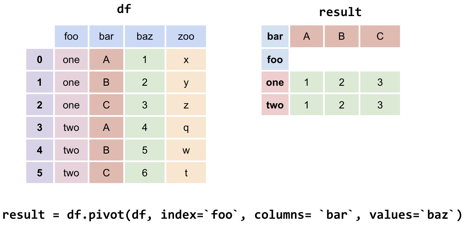
Fig. 1.29 A pivot table is a way of summarizing data in a DataFrame for a particular purpose. It makes heavy use of the aggregation function. A pivot table is itself a DataFrame, where the rows represent one variable that you’re interested in, the columns another, and the cell’s some aggregate value. A pivot table also tends to include marginal values (like sums) for each row and column.

We can even include multiple values in the index or columns of our pivot tables.

names_pivot = names.pivot_table(
    index="Year",     # the rows (turned into index)
    columns="Sex",    # the column values
    values=["Count", "Name"], 
    aggfunc=max,   # group operation
)
names_pivot.head(6)

	Count		Name
Sex	F	M	F	M
Year
1880	7065	9655	Zula	Zeke
1881	6919	8769	Zula	Zeb
1882	8148	9557	Zula	Zed
1883	8012	8894	Zula	Zeno
1884	9217	9388	Zula	Zollie
1885	9128	8756	Zula	Zollie