1.1. Pandas I: Preliminaries

Pandas is a powerful Python library that is widely used in data science and data analysis. It provides data structures and functions that make working with tabular data easy and intuitive.

It is generally accepted in the data science community as the industry- and academia-standard tool for manipulating tabular data.

1.1.1. Dimensionality of Data

Dimensionality, in the context of data, refers to the number of axes or directions in which data can be represented. The most common dimensions are 0, 1, 2, and n.

Scalars (0-dimensional data; values) are single numbers. They can be integers, real numbers, or complex numbers. Scalars are the simplest objects in linear algebra. In Python, we can represent scalars using the built-in int and float data types. For example, 3 and 3.0 are both scalars.

Vectors (1-dimensional data, collection of values) are one-dimensional arrays of scalars. They are used to represent quantities that have both magnitude and direction. In native Python, we can represent vectors using lists or tuples. For example, [1, 2, 3] is a vector.

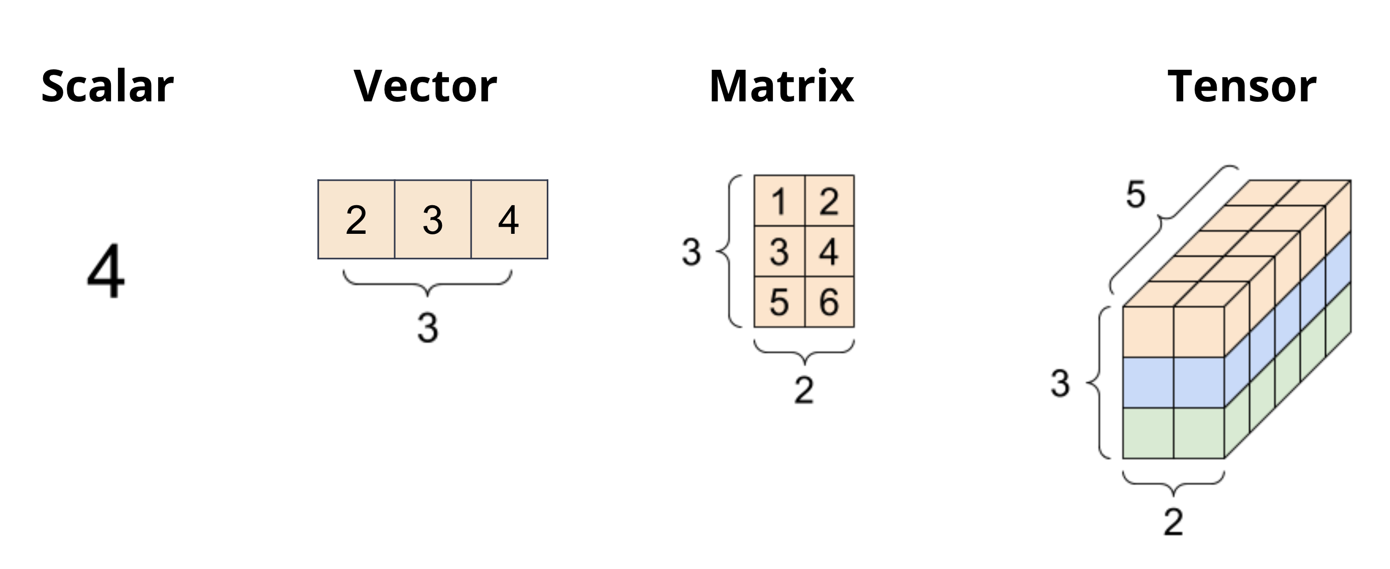
Fig. 1.8 Data can be represented in different dimensions. The most common dimensions are 0, 1, 2, and n.

Matrices (2-dimensional data, collection of vectors) are two-dimensional arrays of scalars. They are used to represent linear transformations from one vector space to another. In native Python, we can represent matrices using lists of lists. For example, [[1, 2], [3, 4]] is a matrix.

Tensors (n-dimensional data, collection of matrices) are n-dimensional arrays of scalars. They are used to represent multi-dimensional data.

1.1.2. Tabular (2-dimensional) Data

Tables are one of the most common ways to organize data. This is in large part due to the simplicity and flexibility of tables. Tables allow us to represent each observation, or instance of collecting data from an individual, as its own row. We can record distinct characteristics, or features, of each observation in separate columns.

Fig. 1.9 A table is a collection of rows and columns. Each row represents an observation, and each column represents a feature of the observation.

To see this in action, we’ll explore the elections dataset, which stores information about political candidates who ran for president of the United States in various years.

The first few rows of elections dataset in CSV format are as follows:

Year,Candidate,Party,Popular vote,Result,%\n
1824,Andrew Jackson,Democratic-Republican,151271,loss,57.21012204\n
1824,John Quincy Adams,Democratic-Republican,113142,win,42.78987796\n
1828,Andrew Jackson,Democratic,642806,win,56.20392707\n
1828,John Quincy Adams,National Republican,500897,loss,43.79607293\n
1832,Andrew Jackson,Democratic,702735,win,54.57478905\n

This dataset is stored in Comma Separated Values (CSV) format. CSV files due to their simplicity and readability are one of the most common ways to store tabular data. Each line in a CSV file (file extension: .csv) represents a row in the table. In other words, each row is separated by a newline character \n. Within each row, each column is separated by a comma ,, hence the name Comma Separated Values.

1.1.3. Reading Data

To begin our studies in pandas, we must first import the library into our Python environment using import pandas as pd statement. pd is a common alias for pandas. The import statement will allow us to use pandas data structures and methods in our code.

Fig. 1.10 Pandas can read from and to a variety of file formats, including CSV, Excel, and SQL databases.

CSV files can be in pandas using read_csv. The following code cell imports pandas as pd, the conventional alias for Pandas and then reads the elections.csv file.

# `pd` is the conventional alias for Pandas
import pandas as pd

url = "https://raw.githubusercontent.com/fahadsultan/csc272/main/data/elections.csv"
elections = pd.read_csv(url)
elections

	Year	Candidate	Party	Popular vote	Result	%
0	1824	Andrew Jackson	Democratic-Republican	151271	loss	57.210122
1	1824	John Quincy Adams	Democratic-Republican	113142	win	42.789878
2	1828	Andrew Jackson	Democratic	642806	win	56.203927
3	1828	John Quincy Adams	National Republican	500897	loss	43.796073
4	1832	Andrew Jackson	Democratic	702735	win	54.574789
...	...	...	...	...	...	...
177	2016	Jill Stein	Green	1457226	loss	1.073699
178	2020	Joseph Biden	Democratic	81268924	win	51.311515
179	2020	Donald Trump	Republican	74216154	loss	46.858542
180	2020	Jo Jorgensen	Libertarian	1865724	loss	1.177979
181	2020	Howard Hawkins	Green	405035	loss	0.255731

182 rows × 6 columns

Let’s dissect the code above.

1. We first import the pandas library into our Python environment, using the alias pd.  import pandas as pd

2. There are a number of ways to read data into a DataFrame. In this course, our datasets are typically stored in a CSV (comma-seperated values) file format. We can import a CSV file into a DataFrame by passing the data path as an argument to the following pandas function.  pd.read_csv("data/elections.csv")

This code stores our DataFrame object in the elections variable. We see that our elections DataFrame has 182 rows and 6 columns (Year, Candidate, Party, Popular Vote, Result, %). Each row represents a single record – in our example, a presedential candidate from some particular year. Each column represents a single attribute, or feature of the record.

In the example above, we constructed a DataFrame object using data from a CSV file. As we’ll explore in the next section, we can also create a DataFrame with data of our own.

In the elections dataset, each row represents one instance of a candidate running for president in a particular year. For example, the first row represents Andrew Jackson running for president in the year 1824. Each column represents one characteristic piece of information about each presidential candidate. For example, the column named Result stores whether or not the candidate won the election.

Some relevant arguments for read_csv are:

• filepath_or_buffer: The path to the CSV file.

• sep: The character that separates the values in the CSV file. By default, this is a comma ,.

• header: The row number to use as the column names. By default, this is 0, which means the first row is used as the column names.

• index_col: The column to use as the row labels of the DataFrame. By default, this is None, which means that the row labels are integers starting from 0.

• error_bad_lines: If True, the parser will skip lines with too many fields rather than raising an error. By default, this is False.

1.1.4. .head() method

.head() is a method of a DataFrame that returns the first n rows of a DataFrame. By default, n is 5. This is useful when you want to quickly check the contents of a DataFrame.

elections.head()

	Year	Candidate	Party	Popular vote	Result	%
0	1824	Andrew Jackson	Democratic-Republican	151271	loss	57.210122
1	1824	John Quincy Adams	Democratic-Republican	113142	win	42.789878
2	1828	Andrew Jackson	Democratic	642806	win	56.203927
3	1828	John Quincy Adams	National Republican	500897	loss	43.796073
4	1832	Andrew Jackson	Democratic	702735	win	54.574789

Similarly, calling df.tail(n) allows us to extract the last n rows of the DataFrame.

elections.tail(3)

	Year	Candidate	Party	Popular vote	Result	%
179	2020	Donald Trump	Republican	74216154	loss	46.858542
180	2020	Jo Jorgensen	Libertarian	1865724	loss	1.177979
181	2020	Howard Hawkins	Green	405035	loss	0.255731

1.1.5. .shape attribute

.shape is an attribute of a DataFrame that returns a tuple representing the dimensions of the DataFrame.

elections.shape

(182, 6)

The first element of the tuple is the number of rows, and the second element is the number of columns.

1.1.6. .dtypes attribute

.dtypes is an attribute of a DataFrame that returns the data type of each column. The data types are returned as a Series with the column names as the index labels.

elections.dtypes

Year              int64
Candidate        object
Party            object
Popular vote      int64
Result           object
%               float64
dtype: object

In pandas, object is the data type used for string columns, while int64 and float64 are used for integer and floating-point columns, respectively.

1.1.7. Writing Data

pandas can also write data to a variety of file formats, including CSV, Excel, and SQL databases. The following code cell writes the elections dataset to a CSV file named elections.csv.

Fig. 1.11 Pandas can write to a variety of file formats, including CSV, Excel, XML, JSON and SQL. To write to a format, use the to_<format> method on a DataFrame with the desired file name as an argument.

pd.to_csv('elections_new.csv')

1.1.8. DataFrame, Series and Index

There are three fundamental data structures in pandas:

1. Series: 1D labeled array data; best thought of as columnar data

2. DataFrame: 2D tabular data with rows and columns

3. Index: A sequence of row/column labels

DataFrames, Series, and Indices can be represented visually in the following diagram, which considers the first few rows of the elections dataset.

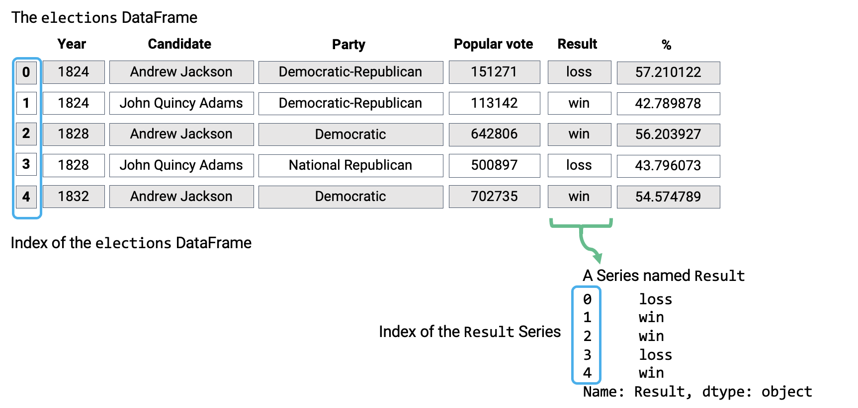
Fig. 1.12 Three fundamental pandas data structures: Series, DataFrame, Index

Notice how the DataFrame is a two-dimensional object – it contains both rows and columns. The Series above is a singular column of this DataFrame, namely, the Result column. Both contain an Index, or a shared list of row labels (here, the integers from 0 to 4, inclusive).

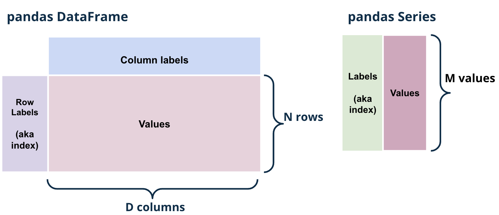
Fig. 1.13 Schematic of a pandas DataFrame and Series

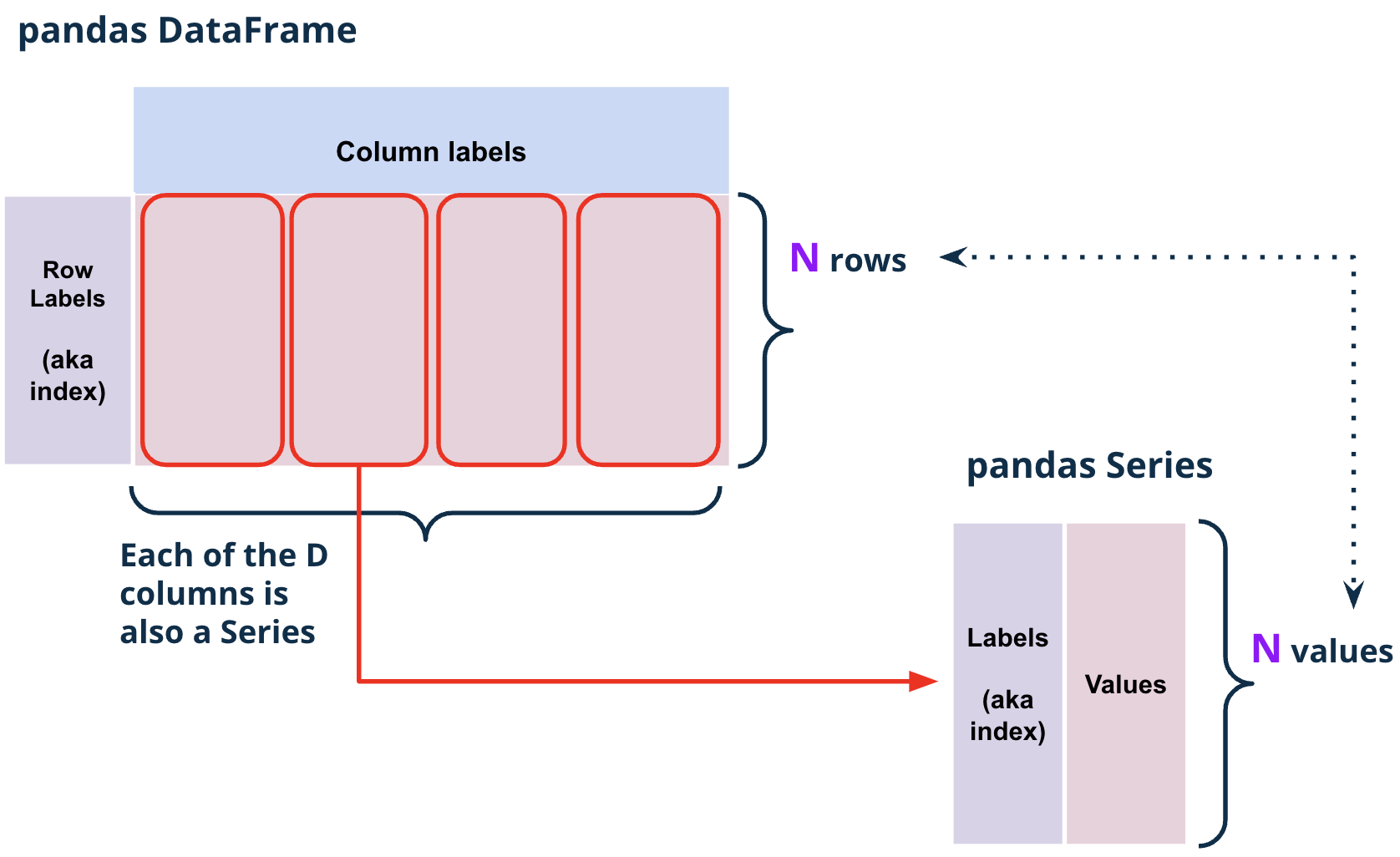
Fig. 1.14 Each column of a pandas DataFrame df is a Series s where s.index == df.index

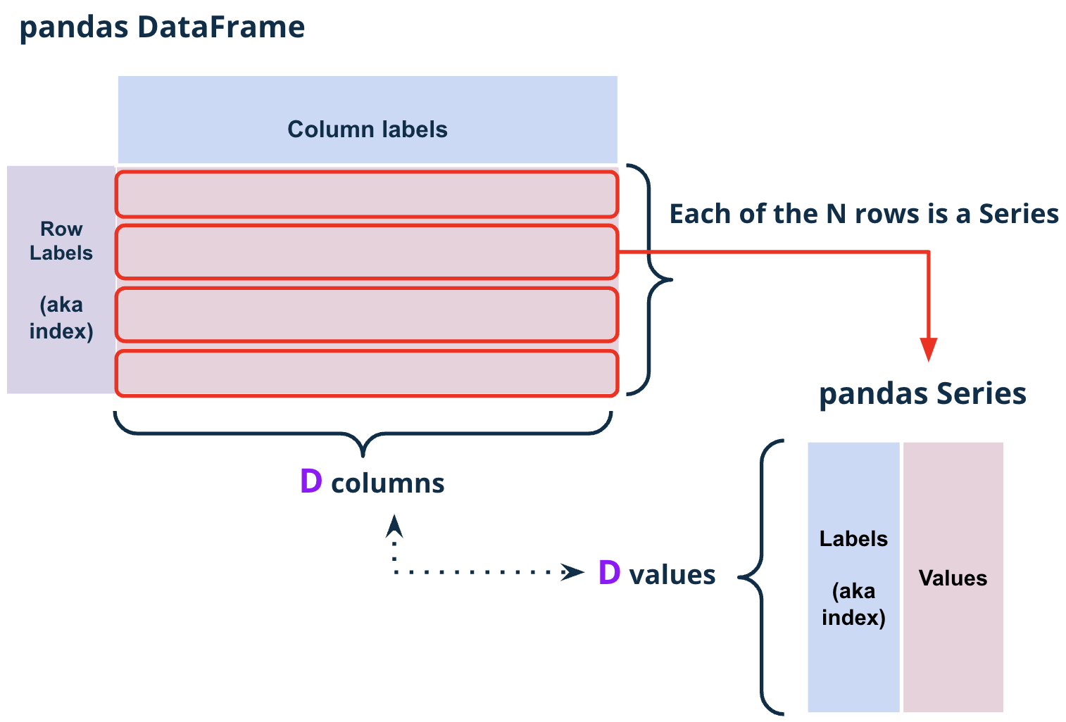
Fig. 1.15 Each row of a pandas DataFrame df is a Series s where s.index == df.columns