1.2. Pandas II - Data Manipulation and Wrangling#
Let’s read in the same elections data from the previous exercise and do some data manipulation and wrangling using pandas.
import pandas as pd
url = "https://raw.githubusercontent.com/fahadsultan/csc272/main/data/elections.csv"
elections = pd.read_csv(url)
1.2.1. Data Alignment#
pandas can make it much simpler to work with objects that have different indexes. For example, when you add objects, if any index pairs are not the same, the respective index in the result will be the union of the index pairs. Let’s look at an example:
s1 = pd.Series([7.3, -2.5, 3.4, 1.5], index=["a", "c", "d", "e"])

s2 = pd.Series([-2.1, 3.6, -1.5, 4, 3.1], index=["a", "c", "e", "f", "g"])

s1, s2, s1 + s2
(a    7.3
 c   -2.5
 d    3.4
 e    1.5
 dtype: float64,
 a   -2.1
 c    3.6
 e   -1.5
 f    4.0
 g    3.1
 dtype: float64,
 a    5.2
 c    1.1
 d    NaN
 e    0.0
 f    NaN
 g    NaN
 dtype: float64)
The internal data alignment introduces missing values in the label locations that don’t overlap. Missing values will then propagate in further arithmetic computations.
In the case of DataFrame, alignment is performed on both rows and columns:
df1 = pd.DataFrame({"A": [1, 2], "B":[3, 4]})
df2 = pd.DataFrame({"B": [5, 6], "D":[7, 8]})
df1 + df2
1.2.2. Math Operations#
In native Python, we have a number of operators that we can use to manipulate data. Most, if not all, of these operators can be used with Pandas Series and DataFrames and are applied element-wise in parallel. A summary of the operators supported by Pandas is shown below:
Category |
Operators |
Supported by Pandas |
Comments |
|---|---|---|---|
Arithmetic |
|
✅ |
Assuming comparable shapes (equal length) |
Assignment |
|
✅ |
Assuming comparable shapes |
Comparison |
|
✅ |
Assuming comparable shapes |
Logical |
|
❌ |
Use |
Identity |
|
✅ |
Assuming comparable data type/structure |
Membership |
|
❌ |
Use |
Bitwise |
|
❌ |
The most significant difference is that logical operators and, or, and not are NOT used with Pandas Series and DataFrames. Instead, we use &, |, and ~ respectively.
Membership operators in and not in are also not used with Pandas Series and DataFrames. Instead, we use the isin() method.
1.2.3. Creating new columns#
Creating new columns in a DataFrame is a common task when working with data. In this notebook, we will see how to create new columns in a DataFrame based on existing columns or other values.

Fig. 1.16 Creating a new column in a DataFrame#
New columns can be created by assigning a value to a new column name. For example, to create a new column named new_column with a constant value 10, we can use the following code:
elections['constant'] = 10

elections.head()
| Year | Candidate | Party | Popular vote | Result | % | constant | |
|---|---|---|---|---|---|---|---|
| 0 | 1824 | Andrew Jackson | Democratic-Republican | 151271 | loss | 57.210122 | 10 |
| 1 | 1824 | John Quincy Adams | Democratic-Republican | 113142 | win | 42.789878 | 10 |
| 2 | 1828 | Andrew Jackson | Democratic | 642806 | win | 56.203927 | 10 |
| 3 | 1828 | John Quincy Adams | National Republican | 500897 | loss | 43.796073 | 10 |
| 4 | 1832 | Andrew Jackson | Democratic | 702735 | win | 54.574789 | 10 |
If we want to create a new column based on an existing column, we can refer to the existing column by its name, within the square brackets, on the right side of the assignment operator. For example, to create a new column named new_column with the values of the existing column column1, we can use the following code:
elections['total_voters'] = ((elections['Popular vote']* 100) / elections['%']).astype(int)

elections.head()
| Year | Candidate | Party | Popular vote | Result | % | constant | total_voters | |
|---|---|---|---|---|---|---|---|---|
| 0 | 1824 | Andrew Jackson | Democratic-Republican | 151271 | loss | 57.210122 | 10 | 264413 |
| 1 | 1824 | John Quincy Adams | Democratic-Republican | 113142 | win | 42.789878 | 10 | 264412 |
| 2 | 1828 | Andrew Jackson | Democratic | 642806 | win | 56.203927 | 10 | 1143702 |
| 3 | 1828 | John Quincy Adams | National Republican | 500897 | loss | 43.796073 | 10 | 1143703 |
| 4 | 1832 | Andrew Jackson | Democratic | 702735 | win | 54.574789 | 10 | 1287655 |
Note that the new column will have the same length as the DataFrame and the calculations are element-wise. That is, the value of the new column at row i will be calculated based on the value of the existing column at row i.

Fig. 1.17 Element-wise operations on existing columns to create a new column#
These element-wise operations are vectorized and are very efficient.
1.2.4. .apply(f, axis=0/1)#
A frequent operation in pandas is applying a function on to either each column or row of a DataFrame.
DataFrame’s apply method does exactly this.

Let’s say we wanted to count the number of unique values that each column takes on. We can use .apply to answer that question:
def count_unique(col):
    return len(set(col))

elections.apply(count_unique, axis="index") # function is passed an individual column
Year             50
Candidate       132
Party            36
Popular vote    182
Result            2
%               182
dtype: int64
1.2.4.1. Column-wise: axis=0 (default)#
data.apply(f, axis=0) applies the function f to each column of the DataFrame data.
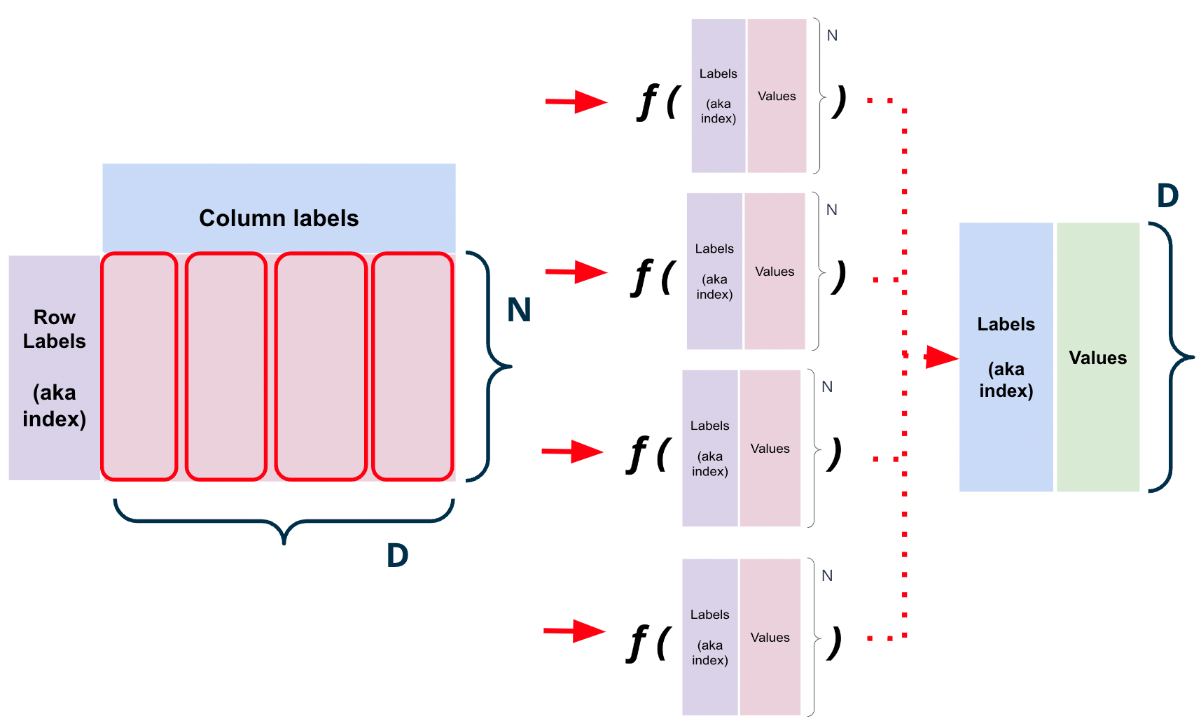
Fig. 1.18 df.apply(f, axis=0) results in \(D\) concurrent calls to \(f\). Each function call is passed a column.#
For example, if we wanted to find the number of unique values in each column of a DataFrame data, we could use the following code:
def count_unique(column):
    return len(column.unique())

elections.apply(count_unique, axis=0)
Year             50
Candidate       132
Party            36
Popular vote    182
Result            2
%               182
dtype: int64
1.2.4.2. Row-wise: axis=1#
data.apply(f, axis=1) applies the function f to each row of the DataFrame data.
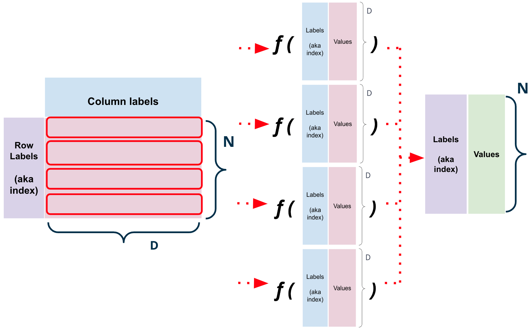
Fig. 1.19 df.apply(f, axis=1) results in \(N\) concurrent calls to \(f\). Each function call is passed a row.#
For instance, let’s say we wanted to count the total number of voters in an election.
We can use .apply to answer that question using the following formula:
def compute_total(row):
    return int(row['Popular vote']*100/row['%'])

elections.apply(compute_total, axis=1)
0         264413
1         264412
2        1143702
3        1143703
4        1287655
         ...
177    135720167
178    158383403
179    158383403
180    158383401
181    158383402
Length: 182, dtype: int64
1.2.5. Summary Statistics#
In data science, we often want to compute summary statistics. pandas provides a number of built-in methods for this purpose.

Fig. 1.20 Aggregating data using one or more operations#
For example, we can use the .mean(), .median() and .std() methods to compute the mean, median, and standard deviation of a column, respectively.
elections['%'].mean(), elections['%'].median(), elections['%'].std()
(27.470350372043967, 37.67789306, 22.96803399144419)
Similarly, we can use the .max() and .min() methods to compute the maximum and minimum values of a Series or DataFrame.
elections['%'].max(), elections['%'].min()
(61.34470329, 0.098088334)
The .sum() method computes the sum of all the values in a Series or DataFrame.

Fig. 1.21 Reduction operations#
The .describe() method computes summary statistics for a Series or DataFrame. It computes the mean, standard deviation, minimum, maximum, and the quantiles of the data.
elections['%'].describe()
count    182.000000
mean      27.470350
std       22.968034
min        0.098088
25%        1.219996
50%       37.677893
75%       48.354977
max       61.344703
Name: %, dtype: float64
elections.describe()
| Year | Popular vote | % | |
|---|---|---|---|
| count | 182.000000 | 1.820000e+02 | 182.000000 |
| mean | 1934.087912 | 1.235364e+07 | 27.470350 |
| std | 57.048908 | 1.907715e+07 | 22.968034 |
| min | 1824.000000 | 1.007150e+05 | 0.098088 |
| 25% | 1889.000000 | 3.876395e+05 | 1.219996 |
| 50% | 1936.000000 | 1.709375e+06 | 37.677893 |
| 75% | 1988.000000 | 1.897775e+07 | 48.354977 |
| max | 2020.000000 | 8.126892e+07 | 61.344703 |
1.2.6. Other Handy Utility Functions#
pandas contains an extensive library of functions that can help shorten the process of setting and getting information from its data structures. In the following section, we will give overviews of each of the main utility functions that will help us in in this course.
Discussing all functionality offered by pandas could take an entire semester! We will walk you through the most commonly-used functions, and encourage you to explore and experiment on your own.
.shape.size.dtypes.astype().describe().sample().value_counts().unique().sort_values()
The pandas documentation will be a valuable resource.
1.2.6.1. .astype()#
Cast a pandas object to a specified dtype
elections['%'].astype(int)
0      57
1      42
2      56
3      43
4      54
       ..
177     1
178    51
179    46
180     1
181     0
Name: %, Length: 182, dtype: int64
1.2.6.2. .describe()#
If many statistics are required from a DataFrame (minimum value, maximum value, mean value, etc.), then .describe() can be used to compute all of them at once.
elections.describe()
| Year | Popular vote | % | |
|---|---|---|---|
| count | 182.000000 | 1.820000e+02 | 182.000000 |
| mean | 1934.087912 | 1.235364e+07 | 27.470350 |
| std | 57.048908 | 1.907715e+07 | 22.968034 |
| min | 1824.000000 | 1.007150e+05 | 0.098088 |
| 25% | 1889.000000 | 3.876395e+05 | 1.219996 |
| 50% | 1936.000000 | 1.709375e+06 | 37.677893 |
| 75% | 1988.000000 | 1.897775e+07 | 48.354977 |
| max | 2020.000000 | 8.126892e+07 | 61.344703 |
A different set of statistics will be reported if .describe() is called on a Series.
elections["Party"].describe()
count            182
unique            36
top       Democratic
freq              47
Name: Party, dtype: object
elections["Popular vote"].describe().astype(int)
count         182
mean     12353635
std      19077149
min        100715
25%        387639
50%       1709375
75%      18977751
max      81268924
Name: Popular vote, dtype: int64
1.2.6.3. .sample()#
As we will see later in the semester, random processes are at the heart of many data science techniques (for example, train-test splits, bootstrapping, and cross-validation). .sample() lets us quickly select random entries (a row if called from a DataFrame, or a value if called from a Series).
By default, .sample() selects entries without replacement. Pass in the argument replace=True to sample with replacement.
# Sample a single row
elections.sample()
| Year | Candidate | Party | Popular vote | Result | % | |
|---|---|---|---|---|---|---|
| 135 | 1988 | George H. W. Bush | Republican | 48886597 | win | 53.518845 |
# Sample 5 random rows
elections.sample(5)
| Year | Candidate | Party | Popular vote | Result | % | |
|---|---|---|---|---|---|---|
| 155 | 2000 | Ralph Nader | Green | 2882955 | loss | 2.741176 |
| 134 | 1984 | Walter Mondale | Democratic | 37577352 | loss | 40.729429 |
| 39 | 1884 | Grover Cleveland | Democratic | 4914482 | win | 48.884933 |
| 84 | 1928 | Herbert Hoover | Republican | 21427123 | win | 58.368524 |
| 177 | 2016 | Jill Stein | Green | 1457226 | loss | 1.073699 |
# Randomly sample 4 names from the year 2000, with replacement
elections[elections["Result"] == "win"].sample(4, replace = True)
| Year | Candidate | Party | Popular vote | Result | % | |
|---|---|---|---|---|---|---|
| 53 | 1896 | William McKinley | Republican | 7112138 | win | 51.213817 |
| 131 | 1980 | Ronald Reagan | Republican | 43903230 | win | 50.897944 |
| 2 | 1828 | Andrew Jackson | Democratic | 642806 | win | 56.203927 |
| 168 | 2012 | Barack Obama | Democratic | 65915795 | win | 51.258484 |
1.2.6.4. .value_counts()#
The Series.value_counts() methods counts the number of occurrence of each unique value in a Series. In other words, it counts the number of times each unique value appears. This is often useful for determining the most or least common entries in a Series.
In the example below, we can determine the name with the most years in which at least one person has taken that name by counting the number of times each name appears in the "Name" column of elections.
elections["Party"].value_counts().head()
Democratic     47
Republican     41
Libertarian    12
Prohibition    11
Socialist      10
Name: Party, dtype: int64
1.2.6.5. .unique()#
If we have a Series with many repeated values, then .unique() can be used to identify only the unique values. Here we return an array of all the names in elections.
elections["Result"].unique()
array(['loss', 'win'], dtype=object)
1.2.6.6. .drop_duplicates()#
If we have a DataFrame with many repeated rows, then .drop_duplicates() can be used to remove the repeated rows.
Where .unique() only works with individual columns (Series) and returns an array of unique values, .drop_duplicates() can be used with multiple columns (DataFrame) and returns a DataFrame with the repeated rows removed.
elections[['Candidate', 'Party']].drop_duplicates()
| Candidate | Party | |
|---|---|---|
| 0 | Andrew Jackson | Democratic-Republican |
| 1 | John Quincy Adams | Democratic-Republican |
| 2 | Andrew Jackson | Democratic |
| 3 | John Quincy Adams | National Republican |
| 5 | Henry Clay | National Republican |
| ... | ... | ... |
| 174 | Evan McMullin | Independent |
| 176 | Hillary Clinton | Democratic |
| 178 | Joseph Biden | Democratic |
| 180 | Jo Jorgensen | Libertarian |
| 181 | Howard Hawkins | Green |
141 rows × 2 columns
1.2.6.7. .sort_values()#
Ordering a DataFrame can be useful for isolating extreme values. For example, the first 5 entries of a row sorted in descending order (that is, from highest to lowest) are the largest 5 values. .sort_values allows us to order a DataFrame or Series by a specified column. We can choose to either receive the rows in ascending order (default) or descending order.
# Sort the "Count" column from highest to lowest
elections.sort_values(by = "%", ascending=False).head()
| Year | Candidate | Party | Popular vote | Result | % | |
|---|---|---|---|---|---|---|
| 114 | 1964 | Lyndon Johnson | Democratic | 43127041 | win | 61.344703 |
| 91 | 1936 | Franklin Roosevelt | Democratic | 27752648 | win | 60.978107 |
| 120 | 1972 | Richard Nixon | Republican | 47168710 | win | 60.907806 |
| 79 | 1920 | Warren Harding | Republican | 16144093 | win | 60.574501 |
| 133 | 1984 | Ronald Reagan | Republican | 54455472 | win | 59.023326 |
We do not need to explicitly specify the column used for sorting when calling .value_counts() on a Series. We can still specify the ordering paradigm – that is, whether values are sorted in ascending or descending order.
# Sort the "Name" Series alphabetically
elections["Candidate"].sort_values(ascending=True).head()
75     Aaron S. Watkins
27      Abraham Lincoln
23      Abraham Lincoln
108     Adlai Stevenson
105     Adlai Stevenson
Name: Candidate, dtype: object
1.2.6.8. .set_index()#
The .set_index() method is used to set the DataFrame index using existing columns.
elections.set_index("Candidate")
| Year | Party | Popular vote | Result | % | |
|---|---|---|---|---|---|
| Candidate | |||||
| Andrew Jackson | 1824 | Democratic-Republican | 151271 | loss | 57.210122 |
| John Quincy Adams | 1824 | Democratic-Republican | 113142 | win | 42.789878 |
| Andrew Jackson | 1828 | Democratic | 642806 | win | 56.203927 |
| John Quincy Adams | 1828 | National Republican | 500897 | loss | 43.796073 |
| Andrew Jackson | 1832 | Democratic | 702735 | win | 54.574789 |
| ... | ... | ... | ... | ... | ... |
| Jill Stein | 2016 | Green | 1457226 | loss | 1.073699 |
| Joseph Biden | 2020 | Democratic | 81268924 | win | 51.311515 |
| Donald Trump | 2020 | Republican | 74216154 | loss | 46.858542 |
| Jo Jorgensen | 2020 | Libertarian | 1865724 | loss | 1.177979 |
| Howard Hawkins | 2020 | Green | 405035 | loss | 0.255731 |
182 rows × 5 columns
1.2.6.9. .reset_index()#
The .reset_index() method is used to reset the index of a DataFrame. By default, the original index is stored in a new column called index.
elections.reset_index()
| index | Year | Candidate | Party | Popular vote | Result | % | |
|---|---|---|---|---|---|---|---|
| 0 | 0 | 1824 | Andrew Jackson | Democratic-Republican | 151271 | loss | 57.210122 |
| 1 | 1 | 1824 | John Quincy Adams | Democratic-Republican | 113142 | win | 42.789878 |
| 2 | 2 | 1828 | Andrew Jackson | Democratic | 642806 | win | 56.203927 |
| 3 | 3 | 1828 | John Quincy Adams | National Republican | 500897 | loss | 43.796073 |
| 4 | 4 | 1832 | Andrew Jackson | Democratic | 702735 | win | 54.574789 |
| ... | ... | ... | ... | ... | ... | ... | ... |
| 177 | 177 | 2016 | Jill Stein | Green | 1457226 | loss | 1.073699 |
| 178 | 178 | 2020 | Joseph Biden | Democratic | 81268924 | win | 51.311515 |
| 179 | 179 | 2020 | Donald Trump | Republican | 74216154 | loss | 46.858542 |
| 180 | 180 | 2020 | Jo Jorgensen | Libertarian | 1865724 | loss | 1.177979 |
| 181 | 181 | 2020 | Howard Hawkins | Green | 405035 | loss | 0.255731 |
182 rows × 7 columns
1.2.6.10. .rename()#
The .rename() method is used to rename the columns or index labels of a DataFrame.
elections.rename(columns={"Candidate":"Name"})
| Year | Name | Party | Popular vote | Result | % | |
|---|---|---|---|---|---|---|
| 0 | 1824 | Andrew Jackson | Democratic-Republican | 151271 | loss | 57.210122 |
| 1 | 1824 | John Quincy Adams | Democratic-Republican | 113142 | win | 42.789878 |
| 2 | 1828 | Andrew Jackson | Democratic | 642806 | win | 56.203927 |
| 3 | 1828 | John Quincy Adams | National Republican | 500897 | loss | 43.796073 |
| 4 | 1832 | Andrew Jackson | Democratic | 702735 | win | 54.574789 |
| ... | ... | ... | ... | ... | ... | ... |
| 177 | 2016 | Jill Stein | Green | 1457226 | loss | 1.073699 |
| 178 | 2020 | Joseph Biden | Democratic | 81268924 | win | 51.311515 |
| 179 | 2020 | Donald Trump | Republican | 74216154 | loss | 46.858542 |
| 180 | 2020 | Jo Jorgensen | Libertarian | 1865724 | loss | 1.177979 |
| 181 | 2020 | Howard Hawkins | Green | 405035 | loss | 0.255731 |
182 rows × 6 columns