1.4. Time Complexity#
Time Complexity of an algorithm is the amount of ‘time’ it takes to run in terms of the size of the input, that is independent of machine and programming language.
In essence, it gives us a way to compare the efficiency and scalability of algorithms.
We can measure this by counting the number of operations that are performed under the assumptions of the RAM model of computation.
1.4.1. Counting Operations#
Consider the following function that takes in a list of numbers and returns the sum of the numbers.
def sum_list(data):
    total = 0
    for num in data:
        total += num
    return total
We can count the number of operations that are performed in this function to get a sense of how long it will take to run. Under the assumptions of RAM model of computation, we assume that each operation that is not a function call or a loop takes 1 unit of time. Using this assumption, we can count the number of operations in the function above as follows:
def sum_list(data):
    total = 0          # 1 operation: assigment
    for num in data:   # n operation where n = len(data)
        total += num   # 2 operations: assignment + addition
    return total       # 1 operation: return
In this case, 2 operations that are performed for each element in the list, so the total number of operations is 2n + 2.
As a general rule, the number of operations in a function is the number of operations in a block of code is:
Please note that this is a rough estimate of the number of operations. The heuristic above assumes a single loop.
In case of multiple loops, we can use the following heuristic for counting the number of operations, for a given pair of loops:
Consider the block of code that follows and answer the Search questions below.
Question: Given two inputs: 1. list of n numbers data and 2. a number called query, return output last location of query in list, if it exists, otherwise return -1
Solution:
def search(data, query):         # 1
   for i in range(len(data)):    # 2
      if data[i] == query:       # 3
         return i                # 4
   return -1                     # 5
1.4.2. Best, Average and Worst Case#
Using the RAM model of computation, we can count how many steps our algorithm takes on any given input instance by executing it.
However, to understand how good or bad an algorithm is in general, we must know how it works over ALL instances (inputs).
To understand the notions of the best, worst, and average-case complexity, think about running an algorithm over all possible instances of data that can be fed to it. For the problem of searching, the set of possible input instances consists of all possible integers as query and all possible lists of \(n\) elements as data.
We can represent each input instance as a point on a graph where the x-axis represents the size of the input problem (size/length of data), and the y-axis denotes the number of steps taken by the algorithm in this instance.
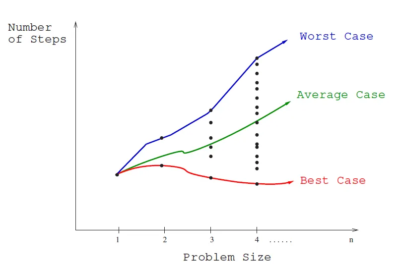
Fig. 1.5 The best, worst, and average-case complexities of an algorithm.#
These points naturally align themselves into columns, because only integers represent possible input size (e.g., it makes no sense to sort 10.57 items). We can define three interesting functions over the plot of these points:
The Worst-case complexity of the algorithm is the function defined by the maximum number of steps taken in any instance of size n. This represents the curve passing through the highest point in each column. This is the blue curve in the figure above.
In case of the search algorithm, the worst case is when the
queryis either not indataor is the last element indata, and the algorithm has to go through all the elements in the list to determine that.The worst-case complexity proves to be most useful of these three measures in practice. The reasons for this is that the worst-case complexity is the highest stakes scenario, and therefore the most important to understand. A lack of understanding and subsequently preparedness for the worst-case scenario can often lead to high cost catastrophic consequences such as downtime, data loss, and even loss of life.
The Best-case complexity of the algorithm is the function defined by the minimum number of steps taken in any instance of size n. This represents the curve passing through the lowest point of each column.
In case of the search algorithm, the best case is when the
queryis the first element indata, and the algorithm only has to go through one element in the list to determine that.In other words, in the best case, the amount of time it takes to run the algorithm is independent of the size of the input.
The best case is rarely used in practice, because it is not a good indicator of how the algorithm will perform in general. In fact, probabilistically speaking, the best case is the least likely to happen.
The Average-case complexity of the algorithm, which is the function defined by the average number of steps over all instances of size n.
In case of the search algorithm, the average case is when the
queryis in the middle ofdata, and the algorithm has to go through half the elements in the list to determine that. This is assuming that thequeryis equally likely to be in any position in the list i.e. incoming queries are uniformly distributed.
The important thing to realize is that each of these time complexities define a numerical function, representing time versus problem size. These functions are as well defined as any other numerical function, be it \(y = x^2 − 2x + 1\) or the price of Google stock as a function of time. But time complexities are such complicated functions that we must simplify them to work with them. For this, we need the “Big Oh” notation and the concept of asymptotic behavior.
1.4.3. \(O\), \(\Omega\), and \(\Theta\)#
Assessing algorithmic performance makes use of the “big Oh” notation that, proves essential to compare algorithms and design more efficient ones.
While the hopelessly “practical” person may blanch at the notion of theoretical analysis, we present the material because it really is useful in thinking about algorithms.
This method of keeping score will be the most mathematically demanding part of this book. But once you understand the intuition behind these ideas, the formalism becomes a lot easier to deal with.
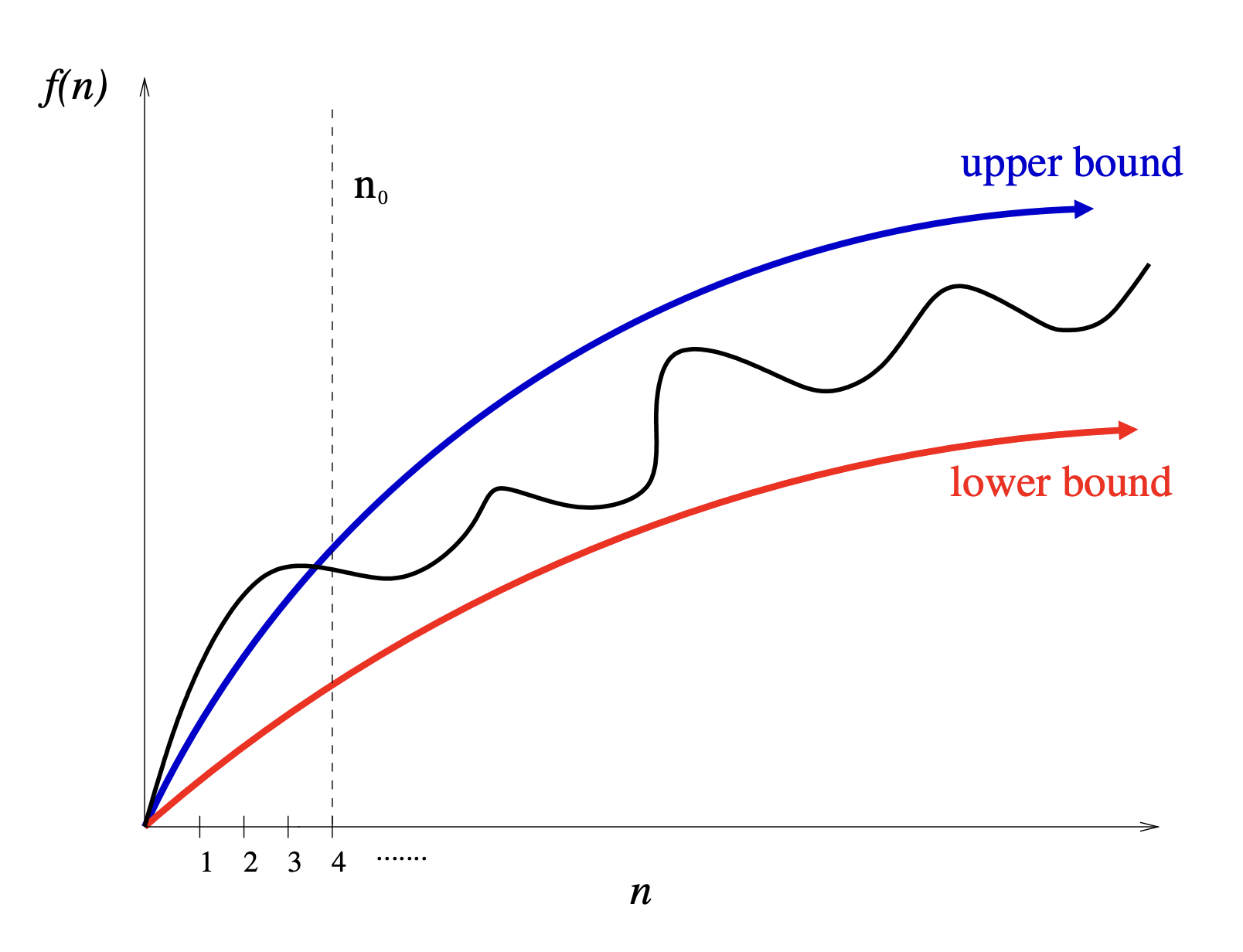
Fig. 1.6 Asymptotic analysis focusing on upper and lower bounds valid for \(n > n_0\) smooth out the bumps of complex functions.#
The best, worst, and average-case time complexities for any given algorithm are numerical functions over the size of possible problem instances. However, it is very difficult to work precisely with these functions, because they tend to:
Have too many bumps – The exact time complexity function for any algorithm is liable to be very complicated with many little up and down bumps as shown in black curve in Figure 7.7. below. This is because the exact number of steps taken by an algorithm depends upon the exact input instance and the space of input instances is wide and varied.
Require too much detail to specify precisely – Counting the exact number of RAM instructions executed in the worst case requires the algorithm be specified to the detail of a complete computer program. Further, the precise answer depends upon uninteresting coding details (e.g., did he use a case statement or nested ifs?). Performing a precise worst-case analysis like
would clearly be very difficult work, but provides us little extra information than the observation that “the time grows quadratically with n.”
It proves to be much easier to talk in terms of simple upper and lower bounds of time-complexity functions using asymptotics. Asymptotic analysis simplifies our analysis by ignoring levels of detail that do not impact our comparison of algorithms.
For example, asymptotic analysis ignores the difference between multiplicative constants. The functions \(f(n) = 2n\) and \(g(n) = n\) are identical in terms of asymptotics. This makes sense given our application. Suppose a given algorithm in (say) C language ran twice as fast as one with the same algorithm written in Java. This multiplicative factor of two tells us nothing about the algorithm itself, since both programs implement exactly the same algorithm. We ignore such constant factors when comparing two algorithms.
1.4.3.1. Formal Definitions#
The formal definitions associated with the Big Oh notation are as follows:
Big Oh \(~O(\cdot)\)
\(f (n) = O(g(n))\) means \(c · g(n)\) is an upper bound on \(f(n)\).
Thus there exists some constant c such that f (n) is always \(\leq c · g(n)\), for large enough \(n\) (i.e. , \(n \geq n_0\) for some constant \(n_0\)).
\(O\) is the function that gives the upper bound on the running time of an algorithm.
For example, our current implementation of
search, we can say that it is \(\O(n)\), since the worst case is when thequeryis either not indataor is the last element indata, and the algorithm has to go through all the elements in the list to determine that, which is dependent on the size of the input.
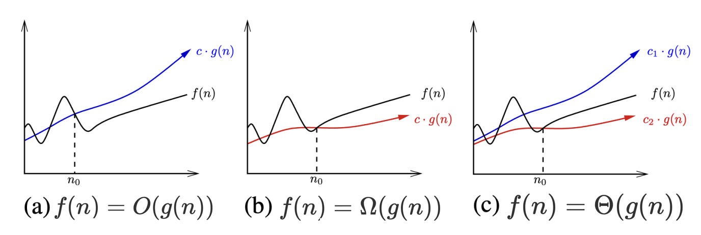
Fig. 1.7 Illustrating the big \(O\), big \(\Omega\), and big \(\Theta\) notations.#
Big Omega \(~\Omega(\cdot)\)
\(f(n) = \Omega(g(n))\) means \(c · g(n)\) is a lower bound on f(n).
Thus there exists some constant \(c\) such that \(f(n)\) is always \(\geq c · g(n)\), for all \(n \geq n_0\).
\(\Omega\) is the function that gives the lower bound on the running time of an algorithm.
For example, our current implementation of
search, we can say that it is \(\Omega(1)\), since the best case is when thequeryis the first element indata, and the algorithm only has to go through one element in the list to determine that, which is independent of the size of the input.
Big Theta \(~\Theta(\cdot)\)
\(f(n) = \Theta(g(n))\) means \(c_1 · g(n)\) is an upper bound on f(n) and \(c_2 · g(n)\) is a lower bound on \(f(n)\), for all \(n \geq n_0\).
Thus there exist constants \(c_1\) and \(c_2\) such that \(f(n) ≤ c_1 · g(n)\) and \(f(n) ≥ \)c_2\( · g(n)\). This means that \(g(n)\) provides a nice, tight bound on f(n).
\(\Theta\) is the function that gives the tight bound on the running time of an algorithm.
For example, our current implementation of
find_max, where the best case is the same as the worst case, we can say that it is \(\Omega(n)\).
These definitions are illustrated in the figure above. Each of these definitions assumes a constant \(n_0\) beyond which they are always satisfied. We are not concerned about small values of \(n\) (i.e. , anything to the left of \(n_0\)). After all, we don’t really care whether one sorting algorithm sorts six items faster than another, but seek which algorithm proves faster when sorting 10,000 or 1,000,000 items. The Big Oh notation enables us to ignore details and focus on the big picture.
1.4.3.2. Informal Usage#
Informally, we can think of \(O(\cdot)\) as the worst-case running time of an algorithm, \(\Omega(\cdot)\) as the best-case running time of an algorithm, and \(\Theta((\cdot))\) as the average-case running time of an algorithm.
That does not mean that we cannot refer to the worst case in terms of Big O. In fact, in practice, we often refer to the best, worst and average case all in terms of Big O.
For instance, we say linear search has worst case time complexity of \(O(n)\), best case time complexity of \(O(1)\), and average case time complexity of \(O(n)\).
1.4.4. Common Time Complexities#
The good news is that only a few function classes tend to occur in the course of basic algorithm analysis. These suffice to cover almost all the algorithms we will discuss in this text, and are listed in order of increasing dominance:
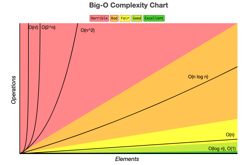
Fig. 1.8 Growth rates of common time complexities.#
Constant functions, \(f(n) = 1\)
Such functions might measure the cost of adding two numbers, printing out “Hello, World!” or the growth realized by functions such as \(f(n) = min(n, 100)\). In the big picture, there is no dependence on the input \(n\).
Logarithmic functions, \(f (n) = log n\)
Logarithmic time-complexity shows up in algorithms such as binary search. Such functions grow quite slowly as n gets big, but faster than the constant function (which is standing still, after all).
Logarithmic algorithms do not loop over all their input, but rather cut the problem size in half at each step. More on logarithms below.
Linear functions, \(f(n) = n\)
Such functions measure the cost of looking at each item once (or twice, or ten times) in an n-element array, say to identify the biggest item, the smallest item, or compute the average value. If your code has a single loop over the input, it is probably linear. Even if your code has more than one loop, it may still be linear as long as no loop is nested inside another.
Superlinear functions, \(f(n) = n lg n\)
This important class of functions arises in such common in-place sorting algorithms. They grow just a little faster than linear, just enough to be a different dominance class. Time complexities of the form \(n lg n\) often result from algorithms that both a) have a loop and b) divide problems in half at each step.
Quadratic functions, \(f(n) = n^2\)
Such functions measure the cost of looking at most or all pairs of items in an n-element universe. This arises in slow sorting algorithms. If your code has two nested loops over the input, it is probably quadratic.
Cubic functions, \(f(n) = n^3\)
Such functions enumerate through all triples of items in an \(n\)-element universe.
These also arise in certain dynamic programming algorithms developed. If your code has three nested loops over the input, it is probably cubic.
Polynomial functions, \(f(n) = n^k\) for a given constant \(k > 1\)
Note that linear, quadratic and cubic functions are all special cases of polynomial functions. Polynomial functions are relevant in Computational Theory and the long unsolved P vs NP problem question.
Polynomial functions arise in algorithms that make multiple passes over the input, such as matrix multiplication. If your code has \(k\) nested loops over the input, it is probably polynomial.
Exponential functions, \(f(n) = c^n\) for a given constant \(c > 1\)
Functions like \(2^n\) arise when enumerating all subsets of n items. Exponential algorithms are uselessly fast.
If your code has \(n\) nested loops over the input, it is probably exponential.
Factorial functions, \(f(n) = n!\)
Functions like \(n!\) arise when generating all permutations or orderings of \(n\) items.
The table below lists the amount of time in seconds for each of the most common time complexities for a given input size \(n\).
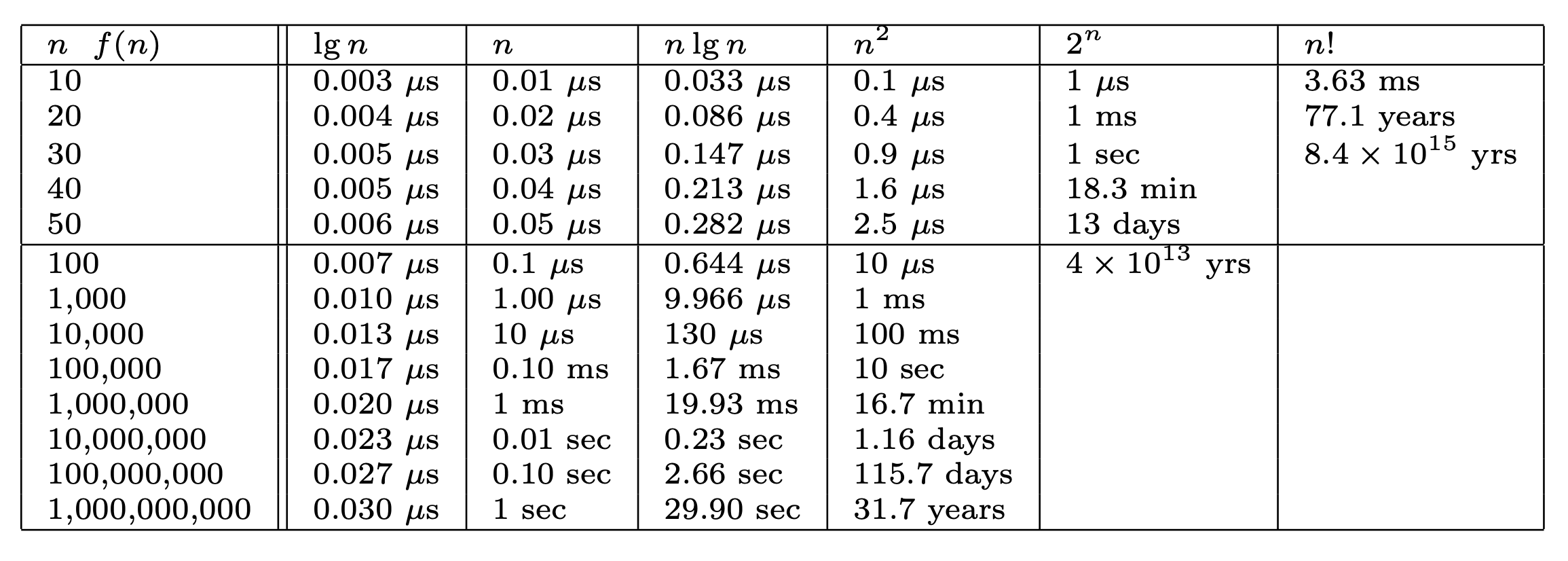
Fig. 1.9 Growth rates of common functions measured in seconds.#
Note that if it takes 1 second for an O(n) algorithm to process 1 billion elements (last row), it takes 31.7 years for an O(\(n^2\)) algorithm to process the same number of elements.
In other words, algorithms with a time complexity worse than \(O(n logn)\) are not at all scalable for any modern day data set.
1.4.5. Logarithms#
Logarithms are the inverse of exponentiation.
In other words, logarithms tell us what power we need to raise a base to in order to get a given number.
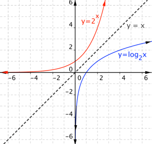
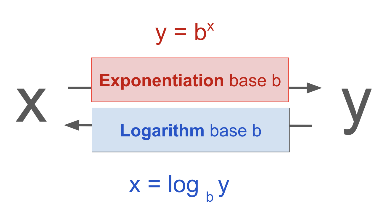
Fig. 1.10 Logarithms are the inverse of exponentiation.#
Where exponentiation grows very quickly, logarithms grow very slowly.
Exponentiation can be thought of as repeated multiplication, and logarithms can be thought of as repeated division.
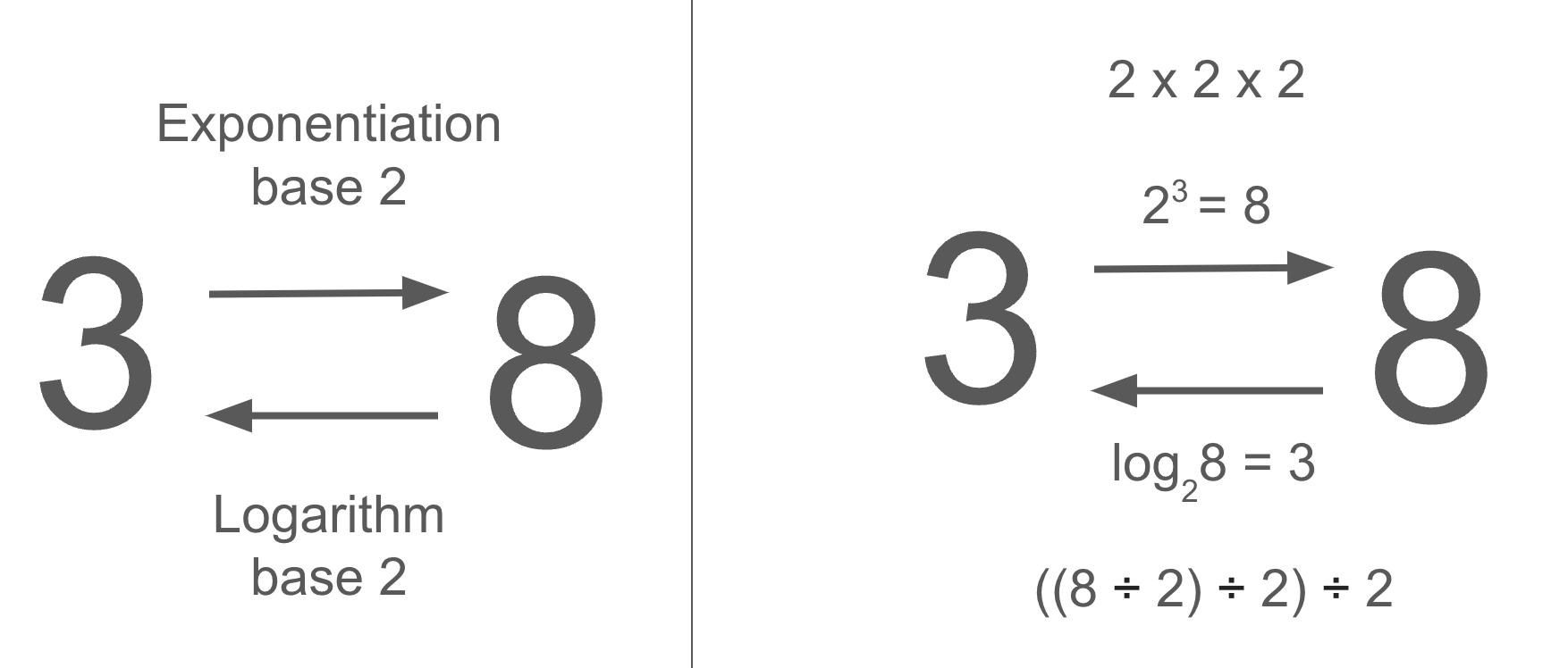
Fig. 1.11 The base of a logarithm is the number that is raised to a power.#
The most common logarithms are base 2, base 10, and base \(e\) (Euler’s number \(\approx\) 2.71828). When base \(e\) is used, the logarithm is called the natural logarithm and is written as \(ln(x)\).
Logarithms are relevant in algorithms because we want our algorithms to scale logarithmically with the size of the input, rather than linearly or worse. Logarithmic algorithms therefore do not iterate over the entire input, but rather divide the input into smaller and smaller pieces, and then solve the problem on each of the pieces.