4.1. Binary Search

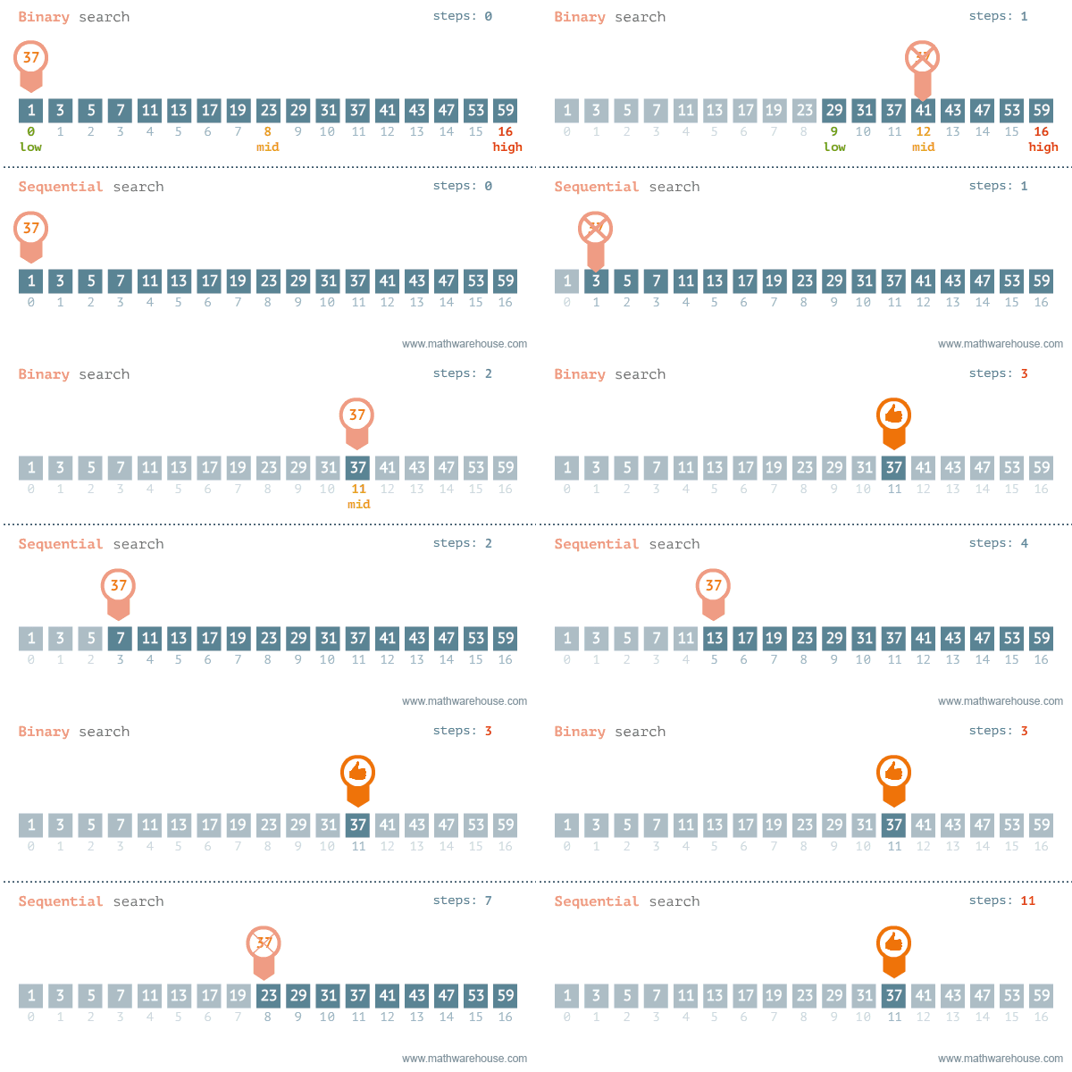
Binary Search is an example of a divide and conquer algorithms. It is a very efficient algorithm for searching through a sorted list. It works by repeatedly dividing the list in half until the target value is found.

The binary search algorithm is a lot like the game “Guess the Number”. In this game, one player thinks of a number between 1 and 100 and the other player tries to guess the number. After each guess, the first player tells the second player if the guess was too high or too low. The second player then uses this information to make a better guess. The second player continues to guess until they find the number.

Fig. 4.2 An animated walkthrough of Binary Search (top) comparing it to Linear / Sequential Search (bottom).

Similarly, the binary search algorithm works similar to how we naturally search for a word in a dictionary. We start by opening the dictionary to the middle. If the word we are looking for is before the word on the page, we open the dictionary to the middle of the left half. If the word we are looking for is after the word on the page, we open the dictionary to the middle of the right half. We continue to divide the dictionary in half until we find the word we are looking for.

Fig. 4.3 A second animated walkthrough of binary search. Note that here the low, mid and high variables are l, m and r.

4.1.1. Algorithm

1. Let $low\leftarrow 0$ and $high\leftarrow n-1$.

2. Compute $mid$ as the average of $low$ and $high$, rounded down (so that it is an integer).

3. If $data[mid]$ equals $query$, then stop. You found it! Return $mid$.

4. If the $mid$ was too low, that is, $data[mid]<query$, then set $low\leftarrow mid+1$.

5. Otherwise, the $mid$ was too high. Set $max\leftarrow mid-1$.

6. Go back to step 2.

Fig. 4.4 This is an example of a binary search steps through time. data = [1,3,4,6,7,8,10,13,14,18,19,21,24,37,40,45,71] and query=7

4.1.2. Pseudocode

Algorithm 4.1 (Binary Search)

Input: A sorted array A[0..n − 1] and a target value Q

Output: an index i such that Q = A[i] or the special value; unsuccessful if no such index exists

1. Set Low to 0 and High to n − 1.

2. If Low > High, the search terminates as unsuccessful.

3. Set Mid (the position of the middle element) to the floor (the largest previous integer) of (Low + High) / 2.

4. If A[Mid] < Q, set Low to Mid + 1 and go to step 2.

5. If A[Mid] > Q, set High to Mid − 1 and go to step 2.

6. Now A[Mid] = T, the search is done; return Mid.

4.1.3. Analysis

The worst-case runtime of binary search is O(log n). The worst case is when the target value is not in the array. In this case, the algorithm will continue to divide the array in half until the subarray is empty. This will take log n iterations.

The best-case runtime of binary search is O(1). The best case is when the target value is the middle element of the array. In this case, the algorithm will find the target on the first iteration.

The average-case runtime of binary search is O(log n). The average case is when the target value is equally likely to be any of the n values in the array. In this case, the algorithm will find the target in log n iterations.

With respect to space, binary search requires O(1) space. This is because the algorithm only needs to store a few integers.