1.5. Space Complexity

Space complexity of an algorithm is the measure of how much extra space we need to allocate in order to run the algorithm.

It is essentially the extra memory required by an algorithm to execute a program and produce output. This includes the memory space used by its inputs, called input space, and any other (auxiliary) memory it uses during execution, which is called auxiliary space.

Similar to time complexity, we talk about the space complexity of an algorithm in terms of its best, worst, and average cases. Of these cases, the worst case is of the most interest. Therefore, similar to time complexity, space complexity is usually expressed in terms of Big O notation.

Consider the following pseudocode for a function that takes in an array of integers and returns the sorted array:

def sort(array):

    copied_array ← make a copy of input array
    
    sorted_array ← new empty list
    
    n ← length of array

    for i ← 0 to n-1:
        
        min_element ← find the minimum element in the copied array
        
        append min_element to sorted_array
        
        remove the minimum element from the copied_array
        
    return sorted_array

Note that the code block above has the space complexity of O(n) since it allocates as much memory for the sorted array as the input array. Additionally, it allocates memory for copying the original input array in order to avoid making any changes/deletions in the original version. In addition, there is memory allocated for min_element variable. Therefore, the algorithm exactly allocates \(2n + 1\) memory, which asymptotically is O(n).

In contrast, consider our original search problem and its solution:

def search(data, query):         # 1
   for i in range(len(data)):    # 2
      if data[i] == query:       # 3
         return i                # 4
   return -1                     # 5

Note that the search function above allocates only memory for i variable. The space complexity of search therefore is constant space: O(1).

Space complexities of most popular and common algorithms belong to an even smaller set of complexities than time complexities.

Most algorithms are either constant space or linear space.

More importantly, while an algorithm of time complexity \(O(n^2)\) with 1 billion rows takes a hopelessly long time to run (about 30 years), an algorithm of space complexity \(O(n^2)\) with 1 billion rows takes only around 1 GB of memory.

To add to that the cost of memory has been decreasing exponentially over the years. The graph below shows the cost of computer memory and storage over time.

Fig. 1.12 Cost of computer memory and storage over time

In computer science, we can often reduce the space complexity of an algorithm at the cost of increasing its time complexity, and vice versa. This is called the space-time tradeoff.

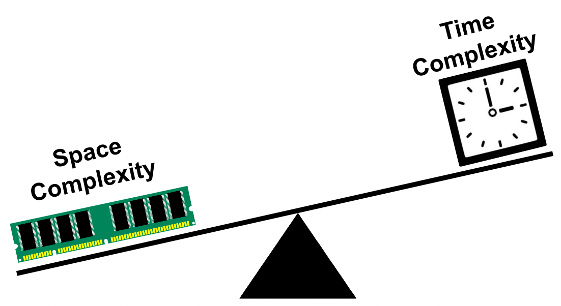
Fig. 1.13 Space Time Tradeoff

In other words, we can often make an algorithm faster by using more space or we can often make an algorithm use less space at the cost of making it slower.

For reasons discussed above, in most real world cases, time complexity is prioritized over space complexity.

An example of this is the use of CDN (Content Delivery Network) by websites. CDNs are used to store a cached version of a website on edge servers in multiple locations around the world. This allows users to access the website from a location that is closest to them, thereby reducing the time it takes to load the website. However, this comes at the cost of using more space to store the cached version of the website.

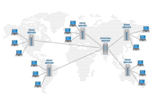
Fig. 1.14 The data on the internet is duplicated and stored on multiple edge servers around the world to reduce the time it takes to load the website. An example of how time/speed is prioritized over space/memory.