5.6. More Recursion

5.6.1. Quick Sort

Recall from Section 4.3. that Quick Sort is a sorting algorithm that uses a divide and conquer strategy. It works by selecting a pivot element from the array and partitioning the other elements into two sub-arrays according to whether they are less than or greater than the pivot. The sub-arrays are then sorted recursively.

This can be done in-place, requiring a constant amount of extra memory and allowing the algorithm to be run in-place. In other words, the space complexity of Quick Sort is O(1) compared to O(n) for Merge Sort.

5.6.1.1. Algorithm

The steps are:

1. Pick an element from the list and call it pivot. This is typically the last element in the list.

2. Partitioning: reorder the list so that all elements with values less than the pivot come before the pivot, while all elements with values greater than the pivot come after it (equal values can go either way). After this partitioning, the pivot is in its final position. This is called the partition operation.

3. Recursively apply the above steps to two sub-lists: one to the left of pivot with elements that all have smaller values and separately to sub-list on the right of pivot containing elements with greater values.

The base case of the recursion are arrays of size zero or one, which are in order by definition, so they never need to be sorted.

The pivot selection and partitioning steps can be done in several different ways; the choice of specific implementation schemes greatly affects the algorithm’s performance.

5.6.1.2. Implementation

The partitioning step, as described in the algorithm, is the most important part of the Quick Sort algorithm. The partitioning step is implemented using the following steps:

1. Initialize pivot to the last element of the array.

2. Initialize left to start of the array and right to the second last element of the array.

3. As the goal is to move all elements less than pivot to the left and all elements greater than pivot to the right, we need to do the following: 3.1. Until the element at left is less than pivot, increment left 3.2. Until the element at right is greater than pivot, decrement right 3.3. If element at left is less than element at right, swap them. 3.4. Continue until left is greater than right.

def partition(data, start, end):

    pivot = data[end]
    left = start
    right = end - 1

    while left < right:

        # move left towards right
        while data[left] < pivot:
            left = left + 1

        # move right towards left
        while right > 0 and data[right] > pivot:
            right = right - 1

        if left < right:
            data[left], data[right] = data[right], data[left]
	
    # insert pivot into its correct place
    data[left], data[end] = data[end], data[left]

    return left

Once we have the partititon function, the Quick Sort algorithm itself is fairly simple.

The basic idea idea is to call partition on data which returns the new location of pivot.

Using the new location of pivot, we recursively call quicksort on the sublists to the left and right of the pivot.

def quicksort(data, low, high):
    if low < high:
        pi = partition(data, low, high)
        quicksort(data, low, pi-1)
        quicksort(data, pi+1, high)

Fig. 5.10 Quicksort diagram. Cells with dark backgrounds represent pivot.
Red boxes correspond to pi = partition(arr, low, high).
Yellow boxes correspond to the first recursive call: quicksort(arr, low, pi-1).
Orange boxes correspond to the second recursive call: quicksort(arr, pi+1, high).

5.6.1.3. Complexity

As discussed before, the space complexity of Quick Sort is O(1) compared to O(n) for Merge Sort since no extra space is required that is dependent on the size of the input.

The worst case time complexity of quick sort is \(O(n^2)\) and the average case time complexity is O(n log n). This is because the worst case occurs when the pivot is the smallest or largest element in the array.

If the pivot is the smallest or largest element, then the partitioning step will only move one element to the left or right of the pivot. This means that the partitioning step will take O(n) time and we will have to do this for every element in the array.

5.6.2. Tower of Hanoi

Tower of Hanoi is a mathematical puzzle where we have three towers (aka rods and pegs) and n disks.

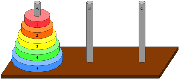
Fig. 5.11 Tower of Hanoi with towers labeled A, B, and C from left to right. There are 5 disks labeled 1 through 5 from top to bottom.

The goal of the puzzle is to move the entire stack of disks from tower A to tower C, obeying the following three simple rules:

1. Only one disk can be moved at a time.

2. A disk can only be moved if it is the uppermost disk on a stack.

3. No disk may be placed on top of a smaller disk.

Fig. 5.12 Optimal solution to Tower of Hanoi problem with 4 disks. The number of steps required to solve a Tower of Hanoi puzzle is \(2^n - 1\), where n is the number of disks.

The puzzle can be played with any number of disks, although many toy versions have around 7 to 9 of them. The minimum number of moves required to solve a Tower of Hanoi puzzle is \(2^n - 1\), where n is the number of disks.

5.6.2.1. Implementation

The Tower of Hanoi is a naturally recursive problem.

The recursive solution is based on the observation that to move n disks from tower A to tower C:

Step 1. We can move n-1 disks from tower A to tower B

Step 2. Then move the nth disk from tower A to tower C

Step 3. Finally move n-1 disks from tower B to tower C.

In python, these recursive steps can be implemented as follows:

def hanoi(n, source="A", buffer="B", destination="C", disk=1):
    """
    Move n disks from source to destination, using buffer, as needed
    """
    
    if n == 1:
        
        print("Move disk", disk, "from", source, "to", destination)

    else:
        
        hanoi(n-1, source="A", buffer="C", destination="B")            # step 1
        hanoi(1,   source="A", buffer="B", destination="C", disk=n)    # step 2
        hanoi(n-1, source="B", buffer="A", destination="C")            # step 3
    
hanoi(3)

Move disk 1 from A to B
Move disk 2 from A to C
Move disk 1 from B to C
Move disk 3 from A to C
Move disk 1 from A to B
Move disk 2 from A to C
Move disk 1 from B to C

The base case of the recursion is when there is only one disk to move. In this case, we simply move the disk from the source tower to the destination tower.

5.6.2.2. Complexity

The time complexity of the Tower of Hanoi is \(O(2^n)\) and the space complexity is O(n).

The time complexity is exponential because the number of moves required to solve the puzzle is \(2^n - 1\), where n is the number of disks.

5.6.2.3. Legend

Accompanying the game was an instruction booklet, describing the game’s purported origins in Tonkin, and claiming that according to legend Brahmins at a temple in Benares have been carrying out the movement of the “Sacred Tower of Brahma”, consisting of 64 golden disks, according to the same rules as in the game, and that the completion of the tower would lead to the end of the world!

If the legend were true, and if the priests were able to move disks at a rate of one per second, using the smallest number of moves, it would take them \(2^{64} − 1\) seconds or roughly 585 billion years to finish, which is about 42 times the estimated current age of the universe 😅.