Divide and Conquer

Niccolò Machiavelli, the famous military strategist, in The Art of War (1521) wrote that a captain should endeavor with every act to divide the forces of the enemy. Machiavelli advises that this act should be achieved either by making him suspicious of his men in whom he trusted, or by giving him cause that he has to separate his forces, and, because of this, become weaker.
In politics, sociology and military strategy, the technique of Divide and Rule refers to the strategy of causing rivalries and fomenting discord amongst rivals and subordinates to maintain control and power. In human history, it has been effectively used to empower the sovereign to control subjects, populations, or quash factions of dissent, who collectively might be able to oppose its rule.
In computer science, however, this technique is used to bring down pesky time and space complexities of inefficient algorithms.
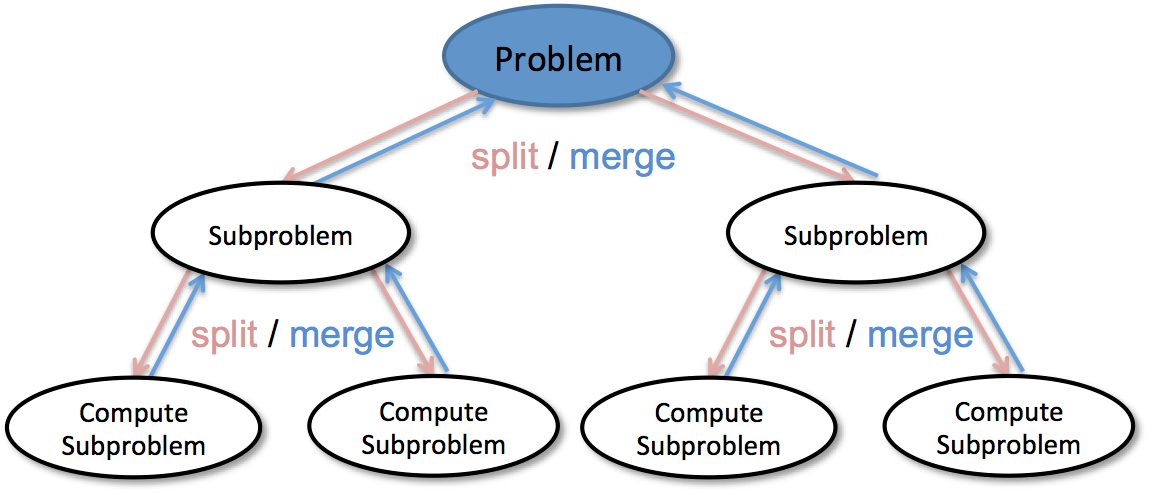
Divide and Conquer is a strategy of solving a problem by breaking the problem into smaller subproblems, solving the subproblems, and combining them to get the desired solution. It is applicable to problems that can be expressed recursively in terms of two or more subproblems of the same or related type, called recurrence relations. The original problem is continually divided into smaller subproblems until these become simple enough to be solved directly. The solutions to the subproblems are then combined to give a solution to the original problem.

For the same problem, divide and conquer algorithms often scale better than their brute force counterparts.
In case of search, where the brute force algorithm is linear $O(n)$, the divide and conquer algorithm is logarithmic $O(\text{log n})$. In case of sorting, where the brute force algorithm is quadratic $O(\text{n}^2)$, the divide and conquer algorithm is log linear $O(\text{n log n})$.
</center>
Binary Search
Binary Search is an example of a divide and conquer algorithms. It is a very efficient algorithm for searching through a sorted list. It works by repeatedly dividing the list in half until the target value is found.
The binary search algorithm is a lot like the game “Guess the Number”. In this game, one player thinks of a number between 1 and 100 and the other player tries to guess the number. After each guess, the first player tells the second player if the guess was too high or too low. The second player then uses this information to make a better guess. The second player continues to guess until they find the number.
Similarly, the binary search algorithm works similar to how we naturally search for a word in a dictionary. We start by opening the dictionary to the middle. If the word we are looking for is before the word on the page, we open the dictionary to the middle of the left half. If the word we are looking for is after the word on the page, we open the dictionary to the middle of the right half. We continue to divide the dictionary in half until we find the word we are looking for.

Algorithm
- Let $low \leftarrow 0$ and $high \leftarrow n-1$.
- Compute $mid$ as the average of $low$ and $high$, rounded down (so that it is an integer).
- If $data[mid]$ equals $query$, then stop. You found it! Return $mid$.
- If the $mid$ was too low, that is, $data[mid] < query$, then set $low \leftarrow mid + 1$.
- Otherwise, the $mid$ was too high. Set $max \leftarrow mid - 1$.
- Go back to step 2.

Implementation
def binary_search(data, query):
	low = 0
	high = len(data) - 1
	while low <= high:
		mid = (low + high) // 2
		if data[mid] == query:
			return mid
		elif data[mid] < query:
			low = mid + 1
		else:
			high = mid - 1
	return -1
Analysis
The worst-case runtime of binary search is O(log n). The worst case is when the target value is not in the array. In this case, the algorithm will continue to divide the array in half until the subarray is empty. This will take log n iterations.
The best-case runtime of binary search is O(1). The best case is when the target value is the middle element of the array. In this case, the algorithm will find the target on the first iteration.
The average-case runtime of binary search is O(log n). The average case is when the target value is equally likely to be any of the n values in the array. In this case, the algorithm will find the target in log n iterations.
With respect to space, binary search requires O(1) space. This is because the algorithm only needs to store a few integers.
Merge Sort
Merge Sort
Merge sort is a divide and conquer algorithm that was invented by John von Neumann in 1945. Merge sort is a comparison sort, meaning that it can sort items of any type for which a “less-than” relation (formally, a total order) is defined.
It is an efficient, general-purpose, comparison-based sorting algorithm. Most implementations produce a stable sort, which means that the order of equal elements is the same in the input and output.
Steps
-
Divide the unsorted list into n sublists, each containing one element (a list of one element is considered sorted).
-
Repeatedly merge sublists to produce new sorted sublists until there is only one sublist remaining. This will be the sorted list.
Implementation
def merge(left, right):
	result = []
	i = j = 0
	while i < len(left) and j < len(right):
		if left[i] < right[j]:
			result.append(left[i])
			i += 1
		else:
			result.append(right[j])
			j += 1
	result.extend(left[i:])
	result.extend(right[j:])
	return result

def merge_sort(data):
	if len(data) <= 1:
		return data
	mid = len(data) // 2
	left = merge_sort(data[:mid])
	right = merge_sort(data[mid:])
	return merge(left, right)
Complexity
The analysis of merge sort can be done in terms of the number of comparisons performed during the sort. This is because every comparison results in a swap, and a swap takes time proportional to the number of items being swapped. The number of comparisons, C(n), performed by a merge sort on n bitonic sequences is bounded by
\[\frac{n}{2} \log_2 n + 2n - \frac{3}{2}\]The number of swaps required by merge sort on n bitonic sequences is bounded by
\[\frac{n}{2} \log_2 n + \frac{n}{2} - 2\]The number of comparisons made by merge sort in the worst case is given by the sorting numbers. The number of comparisons made by merge sort in the average case is given by the sorting numbers. The number of comparisons made by merge sort in the best case is given by the sorting numbers.