1. Pretraining#
1.1. Internet-scale data#
Common Crawl#
Common Crawl is a non-profit organization that crawls the web and freely provides its archives and datasets to the public. It is one of the largest and most comprehensive web crawls available. It has been crawling the web since 2008 and has petabytes (thousands of terabytes) of data.
The code and data are open source and free to use for anyone. Code can be accessed at commoncrawl and the data can be accessed at https://data.commoncrawl.org/.
HuggingFace is a company and open-source community that provides tools and libraries for natural language processing (NLP) and machine learning. They are most well-known for:
Transformers library, which provides pre-trained models for various NLP tasks.
Data Sharing a platform for sharing and discovering datasets, models, and other resources related to NLP.
Model Hub, which hosts thousands of pre-trained models for various NLP tasks.
FineWeb#
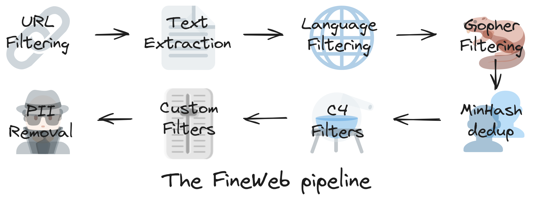
Fineweb is a dataset created by Hugging Face that consists of cleaned and filtered web pages from Common Crawl. It is derived from 96 Common Crawl snapshots. Extensive filtering (boilerplate removal, quality heuristics), deduplication, and cleaning to produce higher-quality web text than raw Common Crawl for FineWeb. It is designed to be used for training large language models. The dataset contains over 1.2 billion web pages, making it one of the largest datasets available for this purpose.
Once cleaned, the data still needs to be compressed into something usable. Instead of feeding raw text into the model, it gets converted into tokens: a structured, numerical representation.
1.2. Tokenization#
Tokenization is the process of breaking raw text (like a sentence or document) into smaller units called tokens that the model can understand.
A token is not always a word. Word-level tokenization struggles with unseen words (“out-of-vocabulary problem”). On the other end, character-level tokenization makes sequences too long.
Byte Pair Encoding (BPE) subword tokenization strikes the right balance. It breaks text into subword units, which can be as small as a single character or as large as a whole word.
For example, the sentence: I love programming! can be tokenized into: ["I", " love", " program", "ming", "!"]
Suppose we have a toy corpus low, lower, newest, widest, the following is how BPE tokenization works:
Start with characters
Represent each word as a sequence of characters plus an end-of-word marker _:
l o w _
l o w e r _
n e w e s t _
w i d e s t _
Count symbol pairs
Find the most frequent adjacent pair of symbols.
“l o” (1), “o w” (2), “w e” (2), “e s” (2), “s t” (2), etc.
Suppose e s is most frequent.
Merge the most frequent pair
Replace e s with a new symbol es:
n e w es t _
w i d es t _
Repeat
Next merge could be
es t → est, thenl o w → low, etc.
Over iterations, you build a vocabulary of subwords.
At the end of the process, Frequent words stay whole and rare words get broken down into smaller, common chunks. You end with a vocabulary that balances:
Size: manageable number of tokens.
Coverage: can represent most words.

You can visualize how this works using tools like Tiktokenizer (https://tiktokenizer.vercel.app).
from collections import Counter

def get_stats(tokens):
    """Count frequency of adjacent symbol pairs in the list of tokens."""
    pairs = Counter()
    for word in tokens:
        for i in range(len(word)-1):
            pairs[(word[i], word[i+1])] += 1
    return pairs

def merge_tokens(tokens, pair):
    """Merge the given pair into a single symbol."""
    new_tokens = []
    bigram = ''.join(pair)
    for word in tokens:
        new_word = []
        i = 0
        while i < len(word):
            # If we find the pair, merge
            if i < len(word)-1 and word[i] == pair[0] and word[i+1] == pair[1]:
                new_word.append(bigram)
                i += 2
            else:
                new_word.append(word[i])
                i += 1
        new_tokens.append(new_word)
    return new_tokens

def byte_pair_encoding(corpus, num_merges=10):
    """Perform BPE on a corpus."""
    # Split words into characters + end-of-word symbol
    tokens = [[c for c in word] + ['</w>'] for word in corpus]

    for _ in range(num_merges):
        pairs = get_stats(tokens)
        if not pairs:
            break
        best = max(pairs, key=pairs.get)
        tokens = merge_tokens(tokens, best)
        print(f"Merged: {best}")
    return tokens

# Example
corpus = ["low", "lower", "lowest"]
final_tokens = byte_pair_encoding(corpus, num_merges=5)

print("Final tokens:")
for t in final_tokens:
    print(t)
LLMs don’t operate directly on raw text. Instead:
Text → tokenizer → tokens (subword units).
Tokens → mapped to integers (IDs in a fixed vocabulary).
These IDs are fed into the model for training or inference.
For reference, GPT-3 uses 50,257 tokens and GPT-4 uses 100,277 tokens in its vocabulary.
1.3. Embeddings#
After BPE, input text is split into subword tokens. Each token is now just an integer ID (index in the vocabulary).
We need to convert these integer IDs into a numerical format that the model can understand. This is where embeddings come in.
An embedding is a dense vector representation of a token in a continuous vector space. Each token is mapped to a high-dimensional vector (e.g., 768, 1024, or even 2048 dimensions). These vectors capture semantic meaning, so similar tokens have similar vectors.
For example, the words “king” and “queen” might have embeddings that are close together in the vector space, while “king” and “car” would be far apart.
Each token ID is then mapped to a dense vector using an embedding matrix E of size [Vocab_size × Embedding_dim]. Suppose Vocab_size = 30,000 and Embedding_dim = 512, then E is a 30,000 × 512 matrix.
If token ID = 421, you take the 421st row of E.
Embeddings are learned during training. The model starts with random vectors for each token and adjusts them based on the context in which the tokens appear. Over time, the embeddings capture relationships between words, such as synonyms, analogies, and more.
import torch
import torch.nn as nn

vocab_size = 30000
embed_dim = 512

embedding_layer = nn.Embedding(vocab_size, embed_dim)

# Example: two BPE tokens
token_ids = torch.tensor([421, 88])  # "jouer" split into two tokens
embeddings = embedding_layer(token_ids)

print(embeddings.shape)  # torch.Size([2, 512])
1.3. Neural Network Training#
Once the data is tokenized, it’s fed into the neural network. More specifically, a Transformer architecture, which is particularly good at handling sequential data like text.
Here’s how that process works:
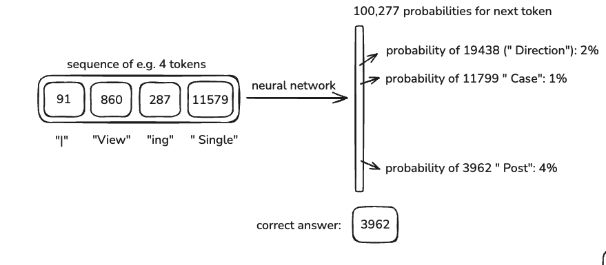
The model takes in a context window, a set number of tokens (e.g., 8,000 for some models, up to 128k for GPT-4).
It predicts the next token based on the patterns it has learned.
The weights in the model are adjusted using backpropagation to reduce errors.
Over time, the model learns to make better predictions.
A longer context window means the model can “remember” more from the input, but it also increases computational cost.
Neural Network Internals
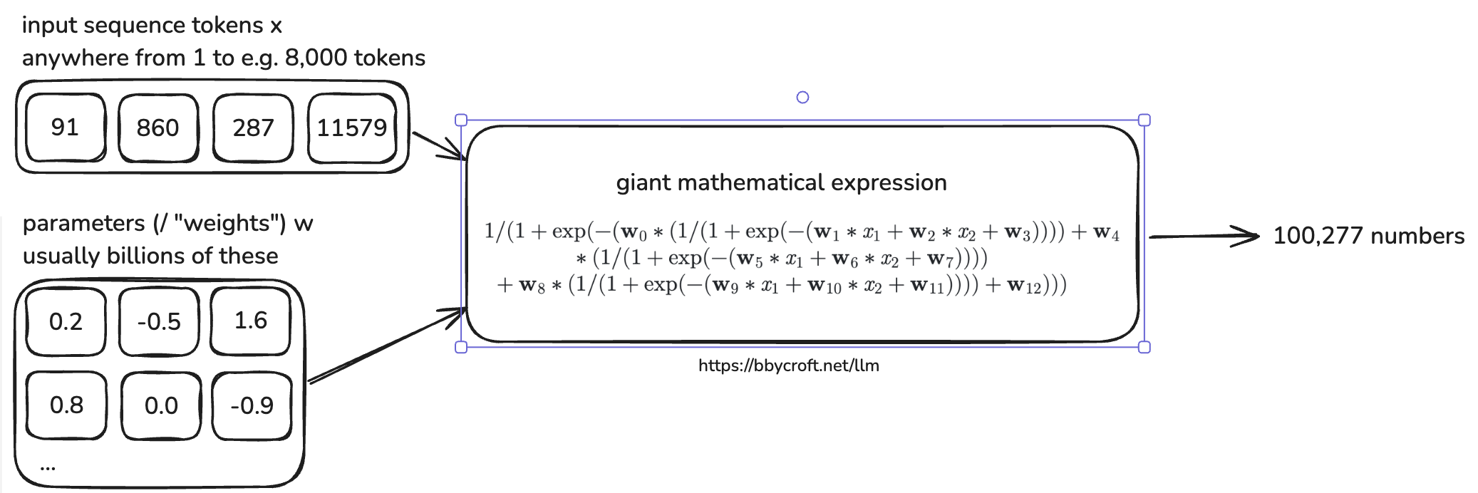
Inside the model, billions of parameters interact with the input tokens to generate a probability distribution for the next token.
This process is defined by complex mathematical equations optimized for efficiency.
Model architectures are designed to balance speed, accuracy, and parallelization.
You can see a production-grade LLM architecture example here.
1.4. Inference#
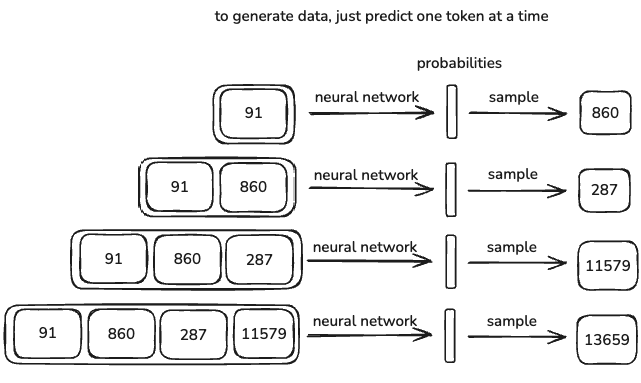
LLMs don’t generate deterministic outputs, they are stochastic. This means the output varies slightly every time you run the model.
The model doesn’t just repeat what it was trained on, it generates responses based on probabilities.
In some cases, the response will match something in the training data exactly, but most of the time, it will generate something new that follows similar patterns.
This randomness is why LLMs can be creative, but also why they sometimes hallucinate incorrect information.
Demo: Reproducing OpenAI’s GPT-2#
GPT-2, released by OpenAI in 2019, was an early example of a transformer-based LLM.
Here’s what it looked like:
1.6 billion parameters
1024-token context length
Trained on ~100 billion tokens
The original GPT-2 training cost was $40,000.
Since then, efficiency has improved dramatically. Andrej Karpathy managed to reproduce GPT-2 using llm.c for just $672. With optimized pipelines, training costs could drop even further to around $100 .
Why is it so much cheaper now?
Better pre-training data extraction techniques → Cleaner datasets mean models learn faster.
Stronger hardware and optimized software → Less computation needed for the same results.
Open Base Models#
Note
The models under discussion do not strictly follow the Open Source Initiative (OSI) definitions of open-source AI (OSI AI Definition). Instead, we use the term open base models to describe models where the weights are publicly accessible, but training data and full reproducibility may not be provided.
Some companies train massive language models (LMs) and release the base models for free. A base model is essentially a raw, pre-trained LM—it still requires fine-tuning or alignment to be practically useful.
Base models are trained on unfiltered internet-scale data, meaning they generate raw completions but lack alignment with human intent.
OpenAI released GPT-2, an open-weight and source-available model, but not fully open-source under OSI’s definition since its training data was not released.
Meta released Llama 3.1 (405B parameters), an open-weight but not open-source model.
To release a base model, two key components are required:
Inference code → Defines the steps the model follows to generate text. Typically written in Python.
Model weights → The billions of parameters that encode the model’s knowledge.
The ‘Psychology’ of Base Models#
Base models can be thoughts of as token-level internet document simulators.
Every run produces a slightly different output (stochastic behavior).
They can regurgitate parts of their training data.
The parameters are like a lossy zip file of internet knowledge.
You can already use them for applications like:
Translation → Using in-context examples.
Basic assistants → Prompting them in a structured way.
Want to experiment with one? Try the Llama 3 (405B base model) here.
At its core, a base model is just an expensive autocomplete. It still needs fine-tuning.