LaTeX#
Note
This tutorial is adapted from Learn LaTeX in 30 minutes
What is LaTeX?#
LaTeX (pronounced “LAY-tek” or “LAH-tek”) is a tool for typesetting professional-looking documents. LaTeX’s mode of operation is quite different from word processors such as Microsoft Word. A LaTeX document is a plain text file interspersed with LaTeX commands used to express the desired (typeset) results.
Typeface vs. Font
A typeface is the underlying visual design that can exist in many different typesetting technologies, and a font is one of these implementations. In other words, a typeface is what you see and a font is what you use.
A font is to typeface what an mp3 file is to a song.
To produce a visible, typeset document, your LaTeX file is processed by a piece of software called a TeX engine which uses the commands embedded in your text file to guide and control the typesetting process, converting the LaTeX commands and document text into a professionally typeset PDF file. This means you only need to focus on the content of your document and the computer, via LaTeX commands and the TeX engine, will take care of the visual appearance (formatting).
The TeX system was developed by the pioneering computer scientist Don Knuth in the 1970s. LaTeX is an extension of TeX, written by Leslie Lamport in the 1980s.
LaTeX markup is widely used in academic circles for publishing papers and books. The strange casing of letters in the name LaTeX was originally to distinguish it from now defunct softwares such as TEX.
The choice of LaTeX or Word depends on the complexity of the document. The more complex it is, the more useful LaTeX will be. These days, most Computer Science publications are written in LaTeX.

Overleaf is a collaborative cloud-based LaTeX editor. Simply put, Overleaf is to LaTeX what Google Docs is to Microsoft Word.
First LaTeX document#
The first step is to start a new project in Overleaf
Let’s start with the simplest working example:
\documentclass{article}
\begin{document}
First document. This is a simple example, with no
extra parameters or packages included.
\end{document}
This example produces the following output:

You can see that LaTeX has automatically indented the first line of the paragraph, taking care of that formatting for you. Let’s have a closer look at what each part of our code does.
The first line of code, \documentclass{article}, declares the document type known as its class, which controls the overall appearance of the document. Different types of documents require different classes; i.e., a CV/resume will require a different class than a scientific paper which might use the standard LaTeX article class. Other types of documents you may be working on may require different classes such as book or report. To get some idea of the many LaTeX class types available, visit the relevant page on CTAN (Comprehensive TeX Archive Network).
Having set the document class, our content, known as the body of the document, is written between the \begin{document} and \end{document} tags. After opening the example above, you can make changes to the text and, when finished, view the resulting typeset PDF by recompiling the document. To do this in Overleaf, simply select the green Recompile button.
Any Overleaf project can be configured to recompile automatically each time it is edited: click the small arrow next to the Recompile button and set Auto Compile to On, as shown in the following screengrab:
Preamble#
When you create a blank project on Overleaf, the LaTeX document is stored as a file called main.tex: the .tex file extension is, by convention, used when naming files containing your document’s LaTeX code.
The previous example showed how document content was entered after the \begin{document} command; however, everything in your .tex file appearing before that point is called the preamble, which acts as the document’s “setup” section. Within the preamble you define the document class (type) together with specifics such as languages to be used when writing the document; loading packages you would like to use (more on this later), and it is where you’d apply other types of configuration.
A minimal document preamble might look like this:
\documentclass[12pt, letterpaper]{article}
\usepackage{graphicx}
where \documentclass[12pt, letterpaper]{article} defines the overall class (type) of document. Additional parameters, which must be separated by commas, are included in square brackets ([...]) and used to configure this instance of the article class; i.e., settings we wish to use for this particular article-class-based document.
In this example, the two parameters do the following:
12pt sets the font size
letterpaper sets the paper size
Of course other font sizes, 9pt, 11pt, 12pt, can be used, but if none is specified, the default size is 10pt. As for the paper size, other possible values are a4paper and legalpaper. For further information see the article about page size and margins.
The preamble line
\usepackage{graphicx}
is an example of loading an external package (here, graphicx) to extend LaTeX’s capabilities, enabling it to import external graphics files. LaTeX packages are discussed in the section Finding and using LaTeX packages.
Title, Author and Date#
Adding a title, author and date to our document requires three more lines in the preamble (not the main body of the document). Those lines are:
\title{My first LaTeX document}: the document title\author{Hubert Farnsworth}: here you write the name of the author(s) and, optionally, the\thankscommand within the curly braces:\thanks{Funded by the Overleaf team.}: can be added after the name of the author, inside the braces of the author command. It will add a superscript and a footnote with the text inside the braces. Useful if you need to thank an institution in your article.
\date{August 2022}: you can enter the date manually or use the command\todayto typeset the current date every time the document is compiled
With these lines added, your preamble should look something like this:
\documentclass[12pt, letterpaper]{article}
\title{My first LaTeX document}
\author{Hubert Farnsworth\thanks{Funded by the Overleaf team.}}
\date{August 2022}
To typeset the title, author and date use the \maketitle command within the body of the document:
\begin{document}
\maketitle
We have now added a title, author and date to our first \LaTeX{} document!
\end{document}
The preamble and body can now be combined to produce a complete document:
\documentclass[12pt, letterpaper]{article}
\title{My first LaTeX document}
\author{Hubert Farnsworth\thanks{Funded by the Overleaf team.}}
\date{August 2022}
\begin{document}
\maketitle
We have now added a title, author and date to our first \LaTeX{} document!
\end{document}
his example produces the following output:

Basic document structure#
Next, we explore abstracts and how to partition a LaTeX document into different chapters, sections and paragraphs.
Abstracts#
Scientific articles usually provide an abstract which is a brief overview/summary of their core topics, or arguments. The next example demonstrates typesetting an abstract using LaTeX’s abstract environment:
\documentclass{article}
\begin{document}
\begin{abstract}
This is a simple paragraph at the beginning of the
document. A brief introduction about the main subject.
\end{abstract}
\end{document}
This example produces the following output:

Paragraphs and new lines#
With the abstract in place, we can begin writing our first paragraph. The next example demonstrates:
how a new paragraph is created by pressing the “enter” key twice, ending the current line and inserting a subsequent blank line;
how to start a new line without starting a new paragraph by inserting a manual line break using the \ command, which is a double backslash; alternatively, use the
\newlinecommand.
The third paragraph in this example demonstrates use of the commands \\ and \newline:
\documentclass{article}
\begin{document}

\begin{abstract}
This is a simple paragraph at the beginning of the
document. A brief introduction about the main subject.
\end{abstract}

After our abstract we can begin the first paragraph, then press ``enter'' twice to start the second one.

This line will start a second paragraph.

I will start the third paragraph and then add \\ a manual line break which causes this text to start on a new line but remains part of the same paragraph. Alternatively, I can use the \verb|\newline|\newline command to start a new line, which is also part of the same paragraph.
\end{document}
This example produces the following output:

Note how LaTeX automatically indents paragraphs—except immediately after document headings such as section and subsection—as we will see.
New users are advised that multiple \\ or \newlines should not used to “simulate” paragraphs with larger spacing between them because this can interfere with LaTeX’s typesetting algorithms. The recommended method is to continue using blank lines for creating new paragraphs, without any \\.
Chapters and sections#
Longer documents, irrespective of authoring software, are usually partitioned into parts, chapters, sections, subsections and so forth. LaTeX also provides document-structuring commands but the available commands, and their implementations (what they do), can depend on the document class being used. By way of example, documents created using the book class can be split into parts, chapters, sections, subsections and so forth but the letter class does not provide (support) any commands to do that.
This next example demonstrates commands used to structure a document based on the book class:
\documentclass{book}
\begin{document}

\chapter{First Chapter}

\section{Introduction}

This is the first section.

Lorem  ipsum  dolor  sit  amet,  consectetuer  adipiscing
elit. Etiam  lobortisfacilisis sem.  Nullam nec mi et
neque pharetra sollicitudin.  Praesent imperdietmi nec ante.
Donec ullamcorper, felis non sodales...

\section{Second Section}

Lorem ipsum dolor sit amet, consectetuer adipiscing elit.
Etiam lobortis facilisissem.  Nullam nec mi et neque pharetra
sollicitudin.  Praesent imperdiet mi necante...

\subsection{First Subsection}
Praesent imperdietmi nec ante. Donec ullamcorper, felis non sodales...

\section*{Unnumbered Section}
Lorem ipsum dolor sit amet, consectetuer adipiscing elit.
Etiam lobortis facilisissem...
\end{document}
This example produces the following output:

The names of sectioning commands are mostly self-explanatory; for example, \chapter{First Chapter} creates a new chapter titled First Chapter, \section{Introduction} produces a section titled Introduction, and so forth. Sections can be further divided into \subsection{...} and even \subsubsection{...}. The numbering of sections, subsections etc. is automatic but can be disabled by using the so-called starred version of the appropriate command which has an asterisk (*) at the end, such as \section*{...} and \subsection*{...}.
Collectively, LaTeX document classes provide the following sectioning commands, with specific classes each supporting a relevant subset:
\part{part}\chapter{chapter}\section{section}\subsection{subsection}\subsubsection{subsubsection}\paragraph{paragraph}\subparagraph{subparagraph}
In particular, the \part and \chapter commands are only available in the report and book document classes.
Visit the Overleaf article article about sections and chapters for further information about document-structure commands.
Bold, italics and underlining#
Next, we will now look at some text formatting commands:
Bold: bold text in LaTeX is typeset using the
\textbf{...}command.Italics: italicised text is produced using the
\textit{...}command.Underline: to underline text use the
\underline{...}command. The next example demonstrates these commands:
Some of the `\textbf{greatest}`
discoveries in \underline{science}
were made by \textbf{\textit{accident}}.
This example produces the following output:

Another very useful command is \emph{argument}, whose effect on its argument depends on the context. Inside normal text, the emphasized text is italicized, but this behaviour is reversed if used inside an italicized text—see the next example:
Some of the greatest \emph{discoveries} in science
were made by accident.

\textit{Some of the greatest \emph{discoveries}
in science were made by accident.}

\textbf{Some of the greatest \emph{discoveries}
in science were made by accident.}
This example produces the following output:

Lists#
You can create different types of list using environments, which are used to encapsulate the LaTeX code required to implement a specific typesetting feature. An environment starts with \begin{environment-name} and ends with \end{environment-name} where environment-name might be figure, tabular or one of the list types: itemize for unordered lists or enumerate for ordered lists.
Unordered lists#
Unordered lists are produced by the itemize environment. Each list entry must be preceded by the \item command, as shown below:
\documentclass{article}
\begin{document}
\begin{itemize}
  \item The individual entries are indicated with a black dot, a so-called bullet.
  \item The text in the entries may be of any length.
\end{itemize}
\end{document}
This example produces the following output:

Ordered lists#
Ordered lists use the same syntax as unordered lists but are created using the enumerate environment:
\documentclass{article}
\begin{document}
\begin{enumerate}
  \item This is the first entry in our list.
  \item The list numbers increase with each entry we add.
\end{enumerate}
\end{document}
This example produces the following output:

As with unordered lists, each entry must be preceded by the \item command which, here, automatically generates the numeric ordered-list label value, starting at 1.
For further information you can open this larger Overleaf project which demonstrates various types of LaTeX list or visit our dedicated help article on LaTeX lists, which provides many more examples and shows how to create customized lists.
Math Equations#
One of the main advantages of LaTeX is the ease with which mathematical expressions can be written. LaTeX provides two writing modes for typesetting mathematics:
inline math mode used for writing formulas that are part of a paragraph
display math mode used to write expressions that are not part of a text or paragraph and are typeset on separate lines
Inline math mode#
Let’s see an example of inline math mode:
\documentclass[12pt, letterpaper]{article}
\begin{document}
In physics, the mass-energy equivalence is stated
by the equation $E=mc^2$, discovered in 1905 by Albert Einstein.
\end{document}
This example produces the following output:

To typeset inline-mode math you can use one of these delimiter pairs: \( ... \), $ ... $ or \begin{math} ... \end{math}, as demonstrated in the following example:
\documentclass[12pt, letterpaper]{article}
\begin{document}
\begin{math}
E=mc^2
\end{math} is typeset in a paragraph using inline math mode---as is $E=mc^2$, and so too is \(E=mc^2\).
\end{document}
This example produces the following output:

Display math mode#
Equations typeset in display mode can be numbered or unnumbered, as in the following example:
\documentclass[12pt, letterpaper]{article}
\begin{document}
The mass-energy equivalence is described by the famous equation
\[ E=mc^2 \] discovered in 1905 by Albert Einstein.

In natural units ($c = 1$), the formula expresses the identity
\begin{equation}
E=m
\end{equation}
\end{document}
This example produces the following output:

To typeset display-mode math you can use one of these delimiter pairs: \[ ... \], \begin{displaymath} ... \end{displaymath} or \begin{equation} ... \end{equation}. Historically, typesetting display-mode math required use of $$ characters delimiters, as in $$ ... display math here ...$$, but this method is no longer recommended: use LaTeX’s delimiters \[ ... \] instead.
The possibilities with math in LaTeX are endless so be sure to visit Overleaf’s help pages for advice and examples on specific topics.
Figures#
In this section we will now look at how to add images to a LaTeX document—note that you need to upload images to your Overleaf project.
The following example demonstrates how to include a picture:
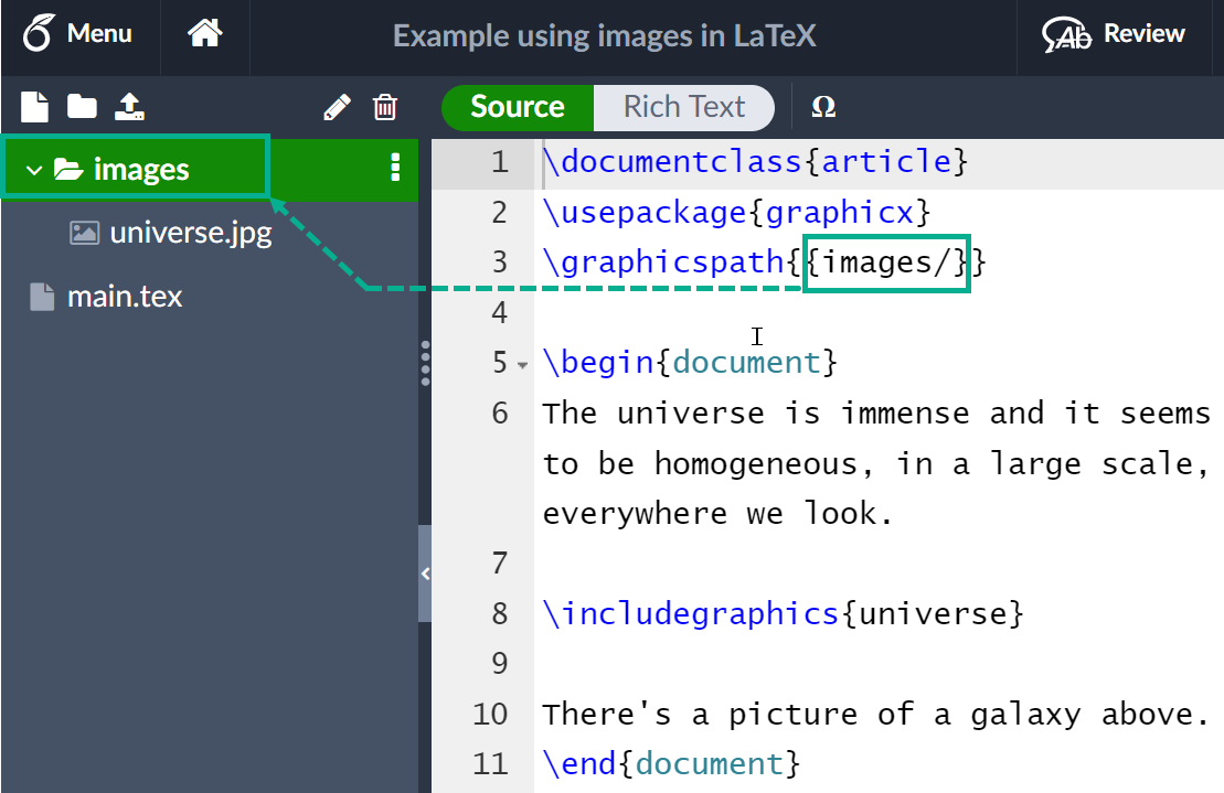
\documentclass{article}
\usepackage{graphicx} %LaTeX package to import graphics
\graphicspath{{images/}} %configuring the graphicx package

\begin{document}
The universe is immense and it seems to be homogeneous,
on a large scale, everywhere we look.

% The \includegraphcs command is
% provided (implemented) by the
% graphicx package
\includegraphics{universe}

There's a picture of a galaxy above.
\end{document}
This example produces the following output:

Importing graphics into a LaTeX document needs an add-on package which provides the commands and features required to include external graphics files. The above example loads the graphicx package which, among many other commands, provides \includegraphics{...} to import graphics and \graphicspath{...} to advise LaTeX where the graphics are located.
To use the graphicx package, include the following line in your Overleaf document preamble:
\usepackage{graphicx}
In our example the command \graphicspath{{images/}} informs LaTeX that images are kept in a folder named images, which is contained in the current directory:
The \includegraphics{universe} command does the actual work of inserting the image in the document. Here, universe is the name of the image file but without its extension.
Note:
Although the full file name, including its extension, is allowed in the
\includegraphicscommand, it’s considered best practice to omit the file extension because it will prompt LaTeX to search for all the supported formats.Generally, the graphic’s file name should not contain white spaces or multiple dots; it is also recommended to use lowercase letters for the file extension when uploading image files to Overleaf.
More information on LaTeX packages can be found at the end of this tutorial in the section Finding and using LaTeX packages.
Captions, labels and references#
Images can be captioned, labelled and referenced by means of the figure environment, as shown below:
\documentclass{article}
\usepackage{graphicx}
\graphicspath{{images/}}

\begin{document}

\begin{figure}[h]
    \centering
    \includegraphics[width=0.75\textwidth]{mesh}
    \caption{A nice plot.}
    \label{fig:mesh1}
\end{figure}

As you can see in figure \ref{fig:mesh1}, the function grows near the origin. This example is on page \pageref{fig:mesh1}.

\end{document}
This example produces the following output:

There are several noteworthy commands in the example:
\includegraphics[width=0.75\textwidth]{mesh}: This form of \includegraphics instructs LaTeX to set the figure’s width to 75% of the text width—whose value is stored in the \textwidth command.\caption{A nice plot.}: As its name suggests, this command sets the figure caption which can be placed above or below the figure. If you create a list of figures this caption will be used in that list.\label{fig:mesh1}: To reference this image within your document you give it a label using the \label command. The label is used to generate a number for the image and, combined with the next command, will allow you to reference it.\ref{fig:mesh1}: This code will be substituted by the number corresponding to the referenced figure.
Images incorporated in a LaTeX document should be placed inside a figure environment, or similar, so that LaTeX can automatically position the image at a suitable location in your document.
Further guidance is contained in the following Overleaf help articles:
Subfigures#
You may want to include some slightly more complicated figures with multiple images. You can do this using subfigure environments inside a figure environment. Before we can do this though, we need to load up the caption and subcaption packages:
\usepackage{caption}
\usepackage{subcaption}
We’ll do an example with three images along side each other with separate captions and labels. Here’s some example code:
\begin{figure}
\centering
\begin{subfigure}[b]{0.3\textwidth}
\centering
\includegraphics[width=\textwidth]{graph1}
\caption{$y=x$}
\label{fig:y equals x}
\end{subfigure}
\hfill
\begin{subfigure}[b]{0.3\textwidth}
\centering
\includegraphics[width=\textwidth]{graph2}
\caption{$y=3\sin x$}
\label{fig:three sin x}
\end{subfigure}
\hfill
\begin{subfigure}[b]{0.3\textwidth}
\centering
\includegraphics[width=\textwidth]{graph3}
\caption{$y=5/x$}
\label{fig:five over x}
\end{subfigure}
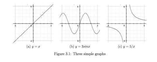
\caption{Three simple graphs}
\label{fig:three graphs}
\end{figure}
To start with, we create a new figure, centre it and then create a new subfigure. In the subfigure command we need to add a placement specifier and then give it a width. Because we want three images next to each other we set a width of 0.3 times the value of \textwidth. You need to make sure that the sum of the widths you specify for the subfigures is less than the text width if you want them all on the same line.
When we add the image in we need to specify the width using width= followed by the \textwidth command. The reason this works is because the text width within the subfigure is the width we specified in the \begin{subfigure} command, i.e. 0.3 times the normal text width (which is the value of \textwidth).
Next we give the subfigure a separate caption and label. We can then end the subfigure and add the next two in. To add some spacing between the figures we’ll use the \hfill command. If you didn’t want them all on the same line you could just leave blank lines instead of the \hfill commands. Please note that the indents I have used do not affect the how the code is processed, they just make it more readable. The beauty of these subfigures is that we can refer to each of them individually in the text due to their individual labels—but we can also give the whole figure a caption and label.
This is what our figure will look like in the document:
Tables#
Tip
Creating tables in LaTeX can be time-consuming so you may want to use the TablesGenerator.com online tool to export LaTeX code for tabulars.
The following examples show how to create tables in LaTeX, including the addition of lines (rules) and captions.
Creating a basic table in \(\LaTeX\)#
We start with an example showing how to typeset a basic table:
\begin{center}
\begin{tabular}{c c c}
 cell1 & cell2 & cell3 \\
 cell4 & cell5 & cell6 \\
 cell7 & cell8 & cell9
\end{tabular}
\end{center}
This example produces the following output:

The tabular environment is the default LaTeX method to create tables. You must specify a parameter to this environment, in this case {c c c} which advises LaTeX that there will be three columns and the text inside each one must be centred. You can also use r to right-align the text and l to left-align it. The alignment symbol & is used to demarcate individual table cells within a table row. To end a table row use the new line command \\. Our table is contained within a center environment to make it centred within the text width of the page.
Adding borders#
The tabular environment supports horizontal and vertical lines (rules) as part of the table:
to add horizontal rules, above and below rows, use the \hline command to add vertical rules, between columns, use the vertical line parameter | In this example the argument is {|c|c|c|} which declares three (centred) columns each separated by a vertical line (rule); in addition, we use \hline to place a horizontal rule above the first row and below the final row:
\begin{center}
\begin{tabular}{|c|c|c|}
 \hline
 cell1 & cell2 & cell3 \\
 cell4 & cell5 & cell6 \\
 cell7 & cell8 & cell9 \\
 \hline
\end{tabular}
\end{center}
This example produces the following output:

Here is a further example:
\begin{center}
 \begin{tabular}{||c c c c||}
 \hline
 Col1 & Col2 & Col2 & Col3 \\ [0.5ex]
 \hline\hline
 1 & 6 & 87837 & 787 \\
 \hline
 2 & 7 & 78 & 5415 \\
 \hline
 3 & 545 & 778 & 7507 \\
 \hline
 4 & 545 & 18744 & 7560 \\
 \hline
 5 & 88 & 788 & 6344 \\ [1ex]
 \hline
\end{tabular}
\end{center}
This example produces the following output:

You can caption and reference tables in much the same way as images. The only difference is that instead of the figure environment, you use the table environment.
Table \ref{table:data} shows how to add a table caption and reference a table.
\begin{table}[h!]
\centering
\begin{tabular}{||c c c c||}
 \hline
 Col1 & Col2 & Col2 & Col3 \\ [0.5ex]
 \hline\hline
 1 & 6 & 87837 & 787 \\
 2 & 7 & 78 & 5415 \\
 3 & 545 & 778 & 7507 \\
 4 & 545 & 18744 & 7560 \\
 5 & 88 & 788 & 6344 \\ [1ex]
 \hline
\end{tabular}
\caption{Table to test captions and labels.}
\label{table:data}
\end{table}
This example produces the following output:

Multiple columns#
Note
Most Computer Science conferences require submitting your work in IEEE format or ACM format. The IEEE format is double column, while the ACM format is single column.
If you are writing a document using two columns (i.e. you started your document with something like \documentclass[twocolumn]{article}).
Page-wide Tables and Figures#
You might have noticed that you can’t use floating elements that are wider than the width of a column (using a LaTeX notation, wider than 0.5\textwidth), otherwise you will see the image overlapping with text. If you really have to use such wide elements, the only solution is to use the “starred” variants of the floating environments, that are {figure*} and {table*}. Those “starred” versions work like the standard ones, but they will be as wide as the page, so you will get no overlapping.
Annoyingly, page-wide elements in a multicolumn document appear on the next page, so you might have to move them around in your document to get them in the right place.
Bibliography#
Bibliography is a list of works such as articles, books, theses, websites, etc. which are referred to in the document.
There are many different ways to maintain bibliographies and cite references in LaTeX. Here, we focus on one of them: using BibTeX.
BibTEX and bibliography database files (.bib files) are extremely useful tools to manage citations and references. We maintain a bibliography database file (let’s name it refs.bib for our example) which contains format-independent information about our references. So our refs.bib file may look like this:
@book{texbook,
  author = {Donald E. Knuth},
  year = {1986},
  title = {The {\TeX} Book},
  publisher = {Addison-Wesley Professional}
}

@book{latex:companion,
  author = {Frank Mittelbach and Michel Gossens
            and Johannes Braams and David Carlisle
            and Chris Rowley},
  year = {2004},
  title = {The {\LaTeX} Companion},
  publisher = {Addison-Wesley Professional},
  edition = {2}
}

@book{latex2e,
  author = {Leslie Lamport},
  year = {1994},
  title = {{\LaTeX}: a Document Preparation System},
  publisher = {Addison Wesley},
  address = {Massachusetts},
  edition = {2}
}

@article{knuth:1984,
  title={Literate Programming},
  author={Donald E. Knuth},
  journal={The Computer Journal},
  volume={27},
  number={2},
  pages={97--111},
  year={1984},
  publisher={Oxford University Press}
}

@inproceedings{lesk:1977,
  title={Computer Typesetting of Technical Journals on {UNIX}},
  author={Michael Lesk and Brian Kernighan},
  booktitle={Proceedings of American Federation of
             Information Processing Societies: 1977
             National Computer Conference},
  pages={879--888},
  year={1977},
  address={Dallas, Texas}
}
You can find more information about other BibTEX reference entry types and fields here — there’s a huge table showing which fields are supported for which entry types. We’ll talk more about how to prepare .bib files in a later section.
Now we can use \cite with the cite keys as before, but now we replace thebibliography with a \bibliographystyle{...} to choose the reference style, as well as \bibliography{...} to point BibTEX at the .bib file where the cited references should be looked-up.
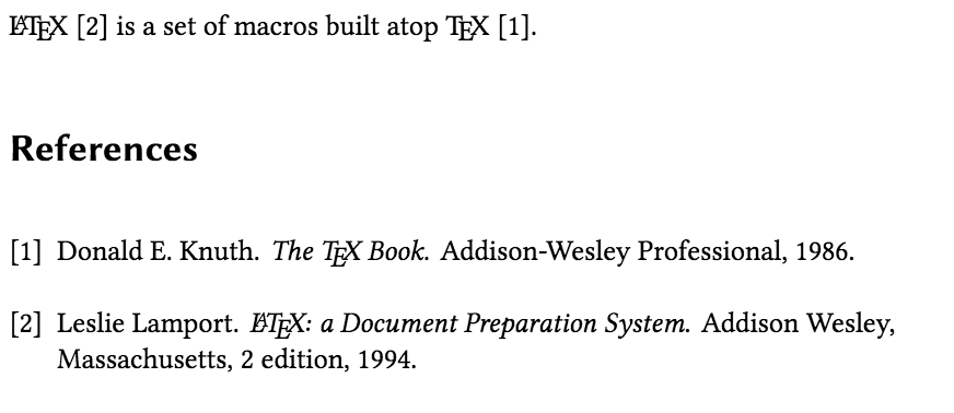
\LaTeX{} \cite{latex2e} is a set of macros built atop \TeX{} \cite{texbook}.
\bibliographystyle{plain} % We choose the "plain" reference style
\bibliography{refs} % Entries are in the refs.bib file
and we get the following output:
Finding bib information#
Note
Google Scholar is not always considered a reliable source of information. For your literature search, you should use the Furman University Library’s academic databases.
Tip
Please reach out to the Outreach Librarian if you need help with your literature search.
Step 1. Go to Google Scholar
Step 2. Search for your topic of interest

Step 3. For the paper you want to cite, click on the quotation mark icon with “Cite” on its right side
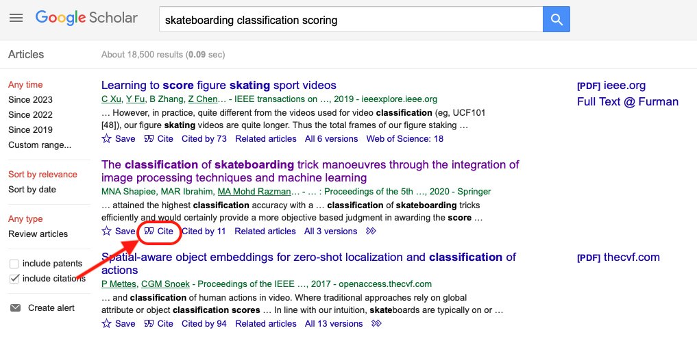
Step 4. From the bottom of the pop-up window, select BibTeX
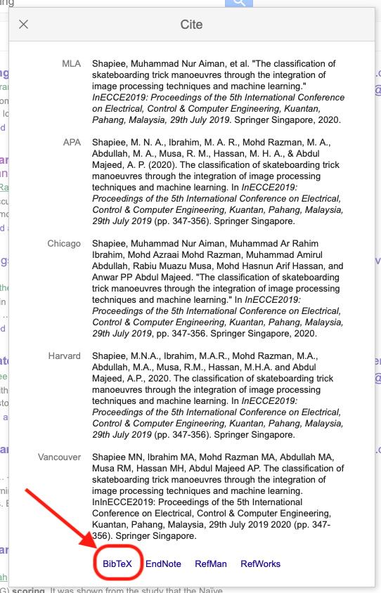
Step 5. You should see a dictionary-like structure with all the meta-data of the publication. Copy the entire text and paste it into your .bib file
@inproceedings{shapiee2020classification,
  title={The classification of skateboarding trick manoeuvres through the integration of image processing techniques and machine learning},
  author={Shapiee, Muhammad Nur Aiman and Ibrahim, Muhammad Ar Rahim and Mohd Razman, Mohd Azraai and Abdullah, Muhammad Amirul and Musa, Rabiu Muazu and Hassan, Mohd Hasnun Arif and Abdul Majeed, Anwar PP},
  booktitle={InECCE2019: Proceedings of the 5th International Conference on Electrical, Control \& Computer Engineering, Kuantan, Pahang, Malaysia, 29th July 2019},
  pages={347--356},
  year={2020},
  organization={Springer}
}
Comments#
LaTeX is a form of “program code”, but one which specializes in document typesetting; consequently, as with code written in any other programming language, it can be very useful to include comments within your document. A LaTeX comment is a section of text that will not be typeset or affect the document in any way—often used to add “to do” notes; include explanatory notes; provide in-line explanations of tricky macros or comment-out lines/sections of LaTeX code when debugging.
To make a comment in LaTeX, simply write a
%symbol at the beginning of the line, as shown in the following code which uses the example above:This example produces output that is identical to the previous LaTeX code which did not contain the comment.